The 10-20-30 Rule and Persistent Poverty Counties
Anti-poverty interventions that provide resources to local communities, based on the characteristics of those communities, have been of interest to Congress. One such policy, dubbed the “10-20-30 rule,” was implemented in the American Recovery and Reinvestment Act of 2009 (ARRA, P.L. 111-5). Title I, Section 105 of ARRA required the Secretary of Agriculture to allocate at least 10% of funds from three rural development program accounts to persistent poverty counties; that is, to counties that have had poverty rates of 20% or more for the past 30 years, as measured by the 1980, 1990, and 2000 decennial censuses. One notable characteristic of this rule is that it did not increase spending for the rural development programs addressed in ARRA, but rather targeted existing funds differently.
Research has suggested that areas for which the poverty rate (the percentage of the population that is below poverty) reaches 20% experience systemic problems that are more acute than in lower-poverty areas. Therefore, policy interventions at the community level (such as applying the 10-20-30 rule to other programs besides those cited in ARRA), and not only at the individual or family level, could continue to be of interest to Congress.
Poverty rates are computed using data from household surveys. Currently, the only data sources that provide poverty estimates for all U.S. counties are the American Community Survey (ACS) and the Small Area Income and Poverty Estimates program (SAIPE); before the mid-1990s, the decennial census was the only source of county poverty estimates. Therefore, to determine whether an area is “persistently” poor in a time span that ends after the year 2000, it must first be decided whether ACS or SAIPE poverty estimates will be used for the later part of that time span.
Lists of persistent poverty counties may differ by roughly 80 to 100 counties in a particular year, depending on the data source selected to compile the list and the rounding method used for the poverty rate estimates. When determining the method to be used to compile a list of persistent poverty counties, the following may be relevant to consider:
Characteristics of interest: SAIPE is suited for poverty or median income alone; ACS for other topics in addition to poverty and income.
Geographic areas of interest: SAIPE is recommended for counties and school districts only; ACS produces estimates for other small geographic areas as well.
Reference period of estimate: SAIPE for one year; ACS for a five-year span.
Rounding method for poverty rates: rounding to 20.0% (one decimal place) yields a shorter list than rounding to 20% (whole number).
Poverty status is not defined for all persons: foster children (unrelated individuals under age 15), institutionalized persons, and residents of college dormitories are excluded; the homeless are not targeted by household surveys; and areas with large numbers of students living off-campus may have high poverty rates.
The 10-20-30 Rule and Persistent Poverty Counties
Jump to Main Text of Report
Contents
- Introduction
- Motivation for Targeting Funds to Persistent Poverty Counties
- Defining "Persistent Poverty" Counties
- Computing the Poverty Rate for an Area
- Data Sources Used in Identifying Persistent Poverty Counties
- Considerations When Identifying and Targeting Persistent Poverty Counties
- Selecting the Data Source: Strengths and Limitations of ACS and SAIPE Poverty Data
- Characteristics of Interest: SAIPE for Poverty Alone; ACS for Other Topics in Addition to Poverty
- Geographic Area of Interest: SAIPE for Counties and School Districts Only; ACS for Other Small Areas
- Reference Period of Estimate: SAIPE for One Year, ACS for a Five-Year Span
- Other Considerations
- Treatment of Special Populations in the Official Poverty Definition
- "Persistence" Versus Flexibility to Recent Situations
- Effects of Rounding and Data Source Selection on Lists of Counties
- Example List of Persistent Poverty Counties
Tables
- Table 1. Number of Counties Identified as Persistently Poor, Using Different Datasets and Rounding Methods
- Table 2. List of Persistent Poverty Counties, Based on 1990 Census, Census 2000, and 2015 Small Area Income and Poverty Estimates (SAIPE), Using Poverty Rates of 19.5% or Greater
- Table A-1. Guidance on Poverty Data Sources by Geographic Level and Type of Estimate
Appendixes
Summary
Anti-poverty interventions that provide resources to local communities, based on the characteristics of those communities, have been of interest to Congress. One such policy, dubbed the "10-20-30 rule," was implemented in the American Recovery and Reinvestment Act of 2009 (ARRA, P.L. 111-5). Title I, Section 105 of ARRA required the Secretary of Agriculture to allocate at least 10% of funds from three rural development program accounts to persistent poverty counties; that is, to counties that have had poverty rates of 20% or more for the past 30 years, as measured by the 1980, 1990, and 2000 decennial censuses. One notable characteristic of this rule is that it did not increase spending for the rural development programs addressed in ARRA, but rather targeted existing funds differently.
Research has suggested that areas for which the poverty rate (the percentage of the population that is below poverty) reaches 20% experience systemic problems that are more acute than in lower-poverty areas. Therefore, policy interventions at the community level (such as applying the 10-20-30 rule to other programs besides those cited in ARRA), and not only at the individual or family level, could continue to be of interest to Congress.
Poverty rates are computed using data from household surveys. Currently, the only data sources that provide poverty estimates for all U.S. counties are the American Community Survey (ACS) and the Small Area Income and Poverty Estimates program (SAIPE); before the mid-1990s, the decennial census was the only source of county poverty estimates. Therefore, to determine whether an area is "persistently" poor in a time span that ends after the year 2000, it must first be decided whether ACS or SAIPE poverty estimates will be used for the later part of that time span.
Lists of persistent poverty counties may differ by roughly 80 to 100 counties in a particular year, depending on the data source selected to compile the list and the rounding method used for the poverty rate estimates. When determining the method to be used to compile a list of persistent poverty counties, the following may be relevant to consider:
- Characteristics of interest: SAIPE is suited for poverty or median income alone; ACS for other topics in addition to poverty and income.
- Geographic areas of interest: SAIPE is recommended for counties and school districts only; ACS produces estimates for other small geographic areas as well.
- Reference period of estimate: SAIPE for one year; ACS for a five-year span.
- Rounding method for poverty rates: rounding to 20.0% (one decimal place) yields a shorter list than rounding to 20% (whole number).
- Poverty status is not defined for all persons: foster children (unrelated individuals under age 15), institutionalized persons, and residents of college dormitories are excluded; the homeless are not targeted by household surveys; and areas with large numbers of students living off-campus may have high poverty rates.
Introduction
Anti-poverty interventions that provide resources to local communities, based on the characteristics of those communities, have been of interest to Congress. One such policy, dubbed the "10-20-30 rule," was implemented in the American Recovery and Reinvestment Act of 2009 (ARRA, P.L. 111-5). Title I, Section 105 of ARRA required the Secretary of Agriculture to allocate at least 10% of funds from three rural development program accounts to persistent poverty counties; that is, to counties that have had poverty rates of 20% or more for the past 30 years, as measured by the 1980, 1990, and 2000 decennial censuses.1
One notable characteristic of this rule is that it did not increase spending for the rural development programs addressed in ARRA, but rather targeted existing funds differently. Given Congress's interest both in addressing poverty and being mindful about levels of federal spending, several bills had been introduced in the 114th Congress that sought to apply the 10-20-30 rule to other programs and in other executive departments.2
This report explains why targeting funds to persistent poverty counties might be of interest, how "persistent poverty" is defined and measured, and how different interpretations of the definition and different data source selections could yield different lists of counties identified as persistently poor. This report does not compare the 10-20-30 rule's advantages and disadvantages against other policy options, nor does it examine the range of programs or policy goals for which the 10-20-30 rule might be an appropriate policy tool.
Motivation for Targeting Funds to Persistent Poverty Counties
Research has suggested that areas for which the poverty rate (the percentage of the population that is below poverty) reaches 20% experience systemic problems that are more acute than in lower-poverty areas. The poverty rate of 20% as a critical point has been discussed in academic literature as relevant for examining social characteristics of high-poverty versus low-poverty areas.3 For instance, property values in high-poverty areas do not yield as high a return on investment as in low-poverty areas, and that low return provides a financial disincentive for property owners to spend money on maintaining and improving property.4 The ill effects of high poverty rates have been documented both for urban and rural areas.5 Therefore, policy interventions at the community level, and not only at the individual or family level, could be of interest to Congress.
Defining "Persistent Poverty" Counties
Computing the Poverty Rate for an Area
Poverty rates are computed by the Census Bureau for the nation, states, and smaller geographic areas such as counties.6 The official definition of poverty in the United States is based on the money income of families and unrelated individuals. Income from each family member (if family members are present) is added together and compared against a dollar amount called a poverty threshold, which represents a level of economic hardship and varies according to the size and characteristics of the family (ranging from one person to nine persons or more). Families (or unrelated individuals) whose income is less than their respective poverty threshold are considered to be in poverty.7
Every person in a family has the same poverty status. Thus, it is possible to compute a poverty rate based on counts of persons (dividing the number of persons below poverty within a county by the county's total population,8 and multiplying by 100 to express as a percentage).
Data Sources Used in Identifying Persistent Poverty Counties
Poverty rates are computed using data from household surveys. Currently, the only data sources that provide poverty estimates for all U.S. counties are the American Community Survey (ACS) and the Small Area Income and Poverty Estimates program (SAIPE). Before the mid-1990s, the only poverty data available at the county level came from the Decennial Census of Population and Housing, which was only collected once every 10 years, and used to be the only source of estimates that could determine whether a county had persistently high poverty rates (ARRA referred explicitly to decennial census poverty estimates for that purpose). However, after Census 2000 the decennial census no longer collects income information, and as a result cannot be used to compute poverty estimates. Therefore, to determine whether an area is persistently poor in a time span that ends after 2000, it must first be decided whether ACS or SAIPE poverty estimates will be used for the later part of that time span.
The ACS and the SAIPE program serve different purposes. The ACS was developed to provide continuous measurement of a wide range of topics similar to that formerly provided by the decennial census long form, available down to the local community level. ACS data for all counties are available annually, but are based on responses over the previous five-year time span (e.g., 2011-2015). The SAIPE program was developed specifically for estimating poverty at the county level for school-age children and for the overall population, for use in funding allocations for the Elementary and Secondary Education Act. SAIPE data are also available annually, and reflect one calendar year, not five. However, unlike the ACS, SAIPE does not provide estimates for a wide array of topics. For further details about the data sources for county poverty estimates, see the Appendix.
Considerations When Identifying and Targeting Persistent Poverty Counties
Selecting the Data Source: Strengths and Limitations of ACS and SAIPE Poverty Data
Because poverty estimates can be obtained from multiple data sources, the Census Bureau has provided guidance on the most suitable data source to use for various purposes.9
Characteristics of Interest: SAIPE for Poverty Alone; ACS for Other Topics in Addition to Poverty
SAIPE poverty estimates are recommended when estimates are needed at the county level, especially for counties with small populations, and when additional demographic and economic detail is not needed at that level.10 When additional detail is required, such as for county-level poverty estimates by race and Hispanic origin, detailed age groups (aside from the elementary and secondary school-age population), housing characteristics, or education level, the ACS is the recommended data source.
Geographic Area of Interest: SAIPE for Counties and School Districts Only; ACS for Other Small Areas
For counties (and school districts) of small population size, SAIPE data have an advantage over ACS data in that the SAIPE model uses administrative data to help reduce the uncertainty of the estimates. However, ACS estimates are available for a wider array of geographic levels, such as ZIP code tabulation areas, census tracts (sub-county areas of roughly 1,200 to 8,000 people), cities and towns, and greater metropolitan areas.
Reference Period of Estimate: SAIPE for One Year, ACS for a Five-Year Span
While the ACS has greater flexibility in the topics measured and the geographic areas provided, it can only provide estimates in five-year ranges for the smallest geographic areas. Five years of survey responses are needed to obtain a sample large enough to produce meaningful estimates for populations below 65,000 persons. In this sense the SAIPE data, because they are based on a single year, are more current than the data of the ACS. The distinction has to do with the reference period of the data—both data sources release data on an annual basis; the ACS estimates for small areas are based on the prior five years, not the prior year alone.
Other Considerations
Treatment of Special Populations in the Official Poverty Definition
Poverty status is not defined for persons in institutions, such as nursing homes or prisons, nor for persons residing in military barracks. These populations are excluded from totals when computing poverty statistics. Furthermore, the homeless population is not counted explicitly in poverty statistics. The ACS is a household survey, thus homeless individuals who are not in shelters are not counted. SAIPE estimates are partially based on Supplemental Nutrition Assistance Program (SNAP) administrative data and tax data, so the part of the homeless population that either filed tax returns or received SNAP benefits might be reflected in the estimates, but only implicitly.
Poverty status also is not defined for persons living in college dormitories. However, students who live in off-campus housing are included. Because college students tend to have lower money income (which does not include school loans) than average, counties that have large populations of students living off-campus may exhibit higher poverty rates than one might expect given other economic measures for the area, such as the unemployment rate.11
Given the ways that the populations above either are or are not reflected in poverty statistics, it may be worthwhile to consider whether counties that have large numbers of people in those populations would receive an equitable allocation of funds. Other economic measures may be of use, depending on the type of program for which funds are being targeted.
"Persistence" Versus Flexibility to Recent Situations
The 10-20-30 rule was developed to identify counties with persistently high poverty rates. Therefore, using that rule by itself would not allow flexibility to target counties that have recently fallen on hard times, such as counties that had a large manufacturing plant close within the past three years. Other interventions besides the 10-20-30 rule may be more appropriate for counties that have had a recent spike in the poverty rate.
Effects of Rounding and Data Source Selection on Lists of Counties
In ARRA, persistent poverty counties were defined as "any county that has had 20 percent or more of its population living in poverty over the past 30 years, as measured by the 1980, 1990, and 2000 decennial censuses."12 Poverty rates published by the Census Bureau are typically reported to one decimal place. The numeral used in the ARRA language was the whole number 20. Thus, for any collection of poverty data, there are two reasonable approaches to compiling a list of persistent poverty counties: using poverty rates of at least 20.0% in all three years, or using poverty rates that round up to the whole number 20% or greater in all three years (i.e., poverty rates of 19.5% or more in all three years). The former approach is more restrictive and results in a shorter list of counties; the latter approach is more inclusive.
Table 1 illustrates the number of counties identified as persistent poverty counties using the 1990 and 2000 decennial censuses, and various ACS and SAIPE datasets for the last data point, under both rounding schemes. The rounding method and data source selection can have a large impact on the number of counties listed. Approximately 30 more counties appear in SAIPE-based lists compared to ACS-based lists using the same rounding method. Compared to using 20.0% as the cutoff (rounded to one decimal place), rounding up to 20% from 19.5% adds approximately 50 counties to the lists based on ACS five-year data, and approximately 60 counties to the lists based on SAIPE data. Taking both the data source and the rounding method together, the list of persistent poverty counties could vary by roughly 80 to 100 counties in a given year depending on the method used.
Table 1. Number of Counties Identified as Persistently Poor, Using Different Datasets and Rounding Methods
Counties identified as having poverty rates of 20% or more (applying rounding methods as indicated below) in 1989 (from 1990 Census), 1999 (from Census 2000), and latest year from datasets indicated below.
|
Dataset |
Rounded to One Decimal Place (20.0% or Greater) |
Rounded to Whole Number (19.5% or Greater) |
Difference Between Rounding Methods |
|
ACS, 2007-2011 |
397 |
445 |
48 |
|
ACS, 2008-2012 |
404 |
456 |
52 |
|
ACS, 2009-2013 |
402 |
458 |
56 |
|
ACS, 2010-2014 |
401 |
456 |
55 |
|
ACS, 2011-2015 |
397 |
453 |
56 |
|
Mean difference: 53.40 |
|||
|
SAIPE, 2011 |
433 |
495 |
62 |
|
SAIPE, 2012 |
435 |
491 |
56 |
|
SAIPE, 2013 |
427 |
490 |
63 |
|
SAIPE, 2014 |
427 |
486 |
59 |
|
SAIPE, 2015 |
419 |
476 |
57 |
|
Mean difference: 59.40 |
|||
|
Differences between datasets released in same year |
|||
|
Difference, SAIPE 2011 minus ACS 2007-2011 |
36 |
50 |
|
|
Difference, SAIPE 2012 minus ACS 2008-2012 |
31 |
35 |
|
|
Difference, SAIPE 2013 minus ACS 2009-2013 |
25 |
32 |
|
|
Difference, SAIPE 2014 minus ACS 2010-2014 |
26 |
30 |
|
|
Difference, SAIPE 2015 minus ACS 2011-2015 |
22 |
23 |
|
|
Mean difference |
28.00 |
34.00 |
Source: Congressional Research Service (CRS) tabulation of data from U.S. Census Bureau, 1990 Census, Census 2000, 2011-2015 Small Area Income and Poverty Estimates, and American Community Survey 5-Year Estimates for 2007-2011, 2008-2012, 2009-2013, 2010-2014, and 2011-2015.
Notes: ACS: American Community Survey. SAIPE: Small Area Income and Poverty Estimates. Comparisons between ACS and SAIPE estimates are between datasets released in the same year (both are typically released in December of the year following the reference period). There are 3,143 county-type areas in the United States.
The selection of the data source and rounding method has a large effect on the number of counties identified as being in persistent poverty. The longest list of persistent poverty counties (SAIPE, 19.5% or greater, that is, rounded up to the whole number 20%) minus the shortest list of persistent poverty counties (ACS, 20.0% or greater) yields the maximum difference. Comparing datasets that were released in the same year, the maximum differences in the lists of counties were
SAIPE 2011, whole number - ACS, 2007-2011, one decimal = 98 counties
SAIPE 2012, whole number - ACS, 2008-2012, one decimal = 87
SAIPE 2013, whole number - ACS, 2009-2013, one decimal = 88
SAIPE 2014, whole number - ACS, 2010-2014, one decimal = 85
SAIPE 2015, whole number - ACS, 2011-2015, one decimal = 79
The lists of persistent poverty counties varied by about 87 counties on average (mean: 87.40), depending on which data source is used for the last data point in the 30-year span, and which rounding method is applied to identify persistent poverty.
Example List of Persistent Poverty Counties
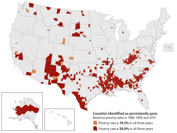
The list of persistent poverty counties below (Table 2) is based on data from the 1990 Census, Census 2000, and the 2015 SAIPE estimates, and included counties with poverty rates of 19.5% or greater (that is, counties with poverty rates that were at least 20% with rounding applied to the whole number). These same counties are mapped in Figure 1.
Table 2. List of Persistent Poverty Counties, Based on 1990 Census, Census 2000, and 2015 Small Area Income and Poverty Estimates (SAIPE), Using Poverty Rates of 19.5% or Greater
|
Count |
FIPS |
State |
County |
Poverty Rate |
Poverty Rate |
Poverty Rate |
|
1 |
01005 |
Alabama |
Barbour |
25.2 |
26.8 |
32.0 |
|
2 |
01007 |
Alabama |
Bibb |
21.2 |
20.6 |
22.2 |
|
3 |
01011 |
Alabama |
Bullock |
36.5 |
33.5 |
39.6 |
|
4 |
01013 |
Alabama |
Butler |
31.5 |
24.6 |
25.8 |
|
5 |
01023 |
Alabama |
Choctaw |
30.2 |
24.5 |
24.4 |
|
6 |
01025 |
Alabama |
Clarke |
25.9 |
22.6 |
22.2 |
|
7 |
01035 |
Alabama |
Conecuh |
29.7 |
26.6 |
28.3 |
|
8 |
01041 |
Alabama |
Crenshaw |
24.3 |
22.1 |
19.9 |
|
9 |
01047 |
Alabama |
Dallas |
36.2 |
31.1 |
34.6 |
|
10 |
01053 |
Alabama |
Escambia |
28.1 |
20.9 |
24.4 |
|
11 |
01061 |
Alabama |
Geneva |
19.5 |
19.6 |
22.4 |
|
12 |
01063 |
Alabama |
Greene |
45.6 |
34.3 |
37.7 |
|
13 |
01065 |
Alabama |
Hale |
35.6 |
26.9 |
28.5 |
|
14 |
01081 |
Alabama |
Lee |
24.9 |
21.8 |
21.0 |
|
15 |
01085 |
Alabama |
Lowndes |
38.6 |
31.4 |
35.2 |
|
16 |
01087 |
Alabama |
Macon |
34.5 |
32.8 |
32.2 |
|
17 |
01091 |
Alabama |
Marengo |
30.0 |
25.9 |
23.3 |
|
18 |
01099 |
Alabama |
Monroe |
22.7 |
21.3 |
28.6 |
|
19 |
01105 |
Alabama |
Perry |
42.6 |
35.4 |
40.0 |
|
20 |
01107 |
Alabama |
Pickens |
28.9 |
24.9 |
24.3 |
|
21 |
01109 |
Alabama |
Pike |
27.2 |
23.1 |
25.9 |
|
22 |
01113 |
Alabama |
Russell |
20.4 |
19.9 |
23.0 |
|
23 |
01119 |
Alabama |
Sumter |
39.7 |
38.7 |
33.2 |
|
24 |
01131 |
Alabama |
Wilcox |
45.2 |
39.9 |
33.2 |
|
25 |
02050 |
Alaska |
Bethel Census Area |
30.0 |
20.6 |
24.2 |
|
26 |
02070 |
Alaska |
Dillingham Census Area |
24.6 |
21.4 |
20.0 |
|
27 |
02158 |
Alaska |
Kusilvak Census Areaa |
31.0 |
26.2 |
31.8 |
|
28 |
02290 |
Alaska |
Yukon-Koyukuk Census Area |
26.0 |
23.8 |
23.4 |
|
29 |
04001 |
Arizona |
Apache |
47.1 |
37.8 |
38.0 |
|
30 |
04009 |
Arizona |
Graham |
26.7 |
23.0 |
22.9 |
|
31 |
04012 |
Arizona |
La Paz |
28.2 |
19.6 |
22.2 |
|
32 |
04017 |
Arizona |
Navajo |
34.7 |
29.5 |
28.1 |
|
33 |
04023 |
Arizona |
Santa Cruz |
26.4 |
24.5 |
24.4 |
|
34 |
05011 |
Arkansas |
Bradley |
24.9 |
26.3 |
28.0 |
|
35 |
05017 |
Arkansas |
Chicot |
40.4 |
28.6 |
31.4 |
|
36 |
05027 |
Arkansas |
Columbia |
24.4 |
21.1 |
23.8 |
|
37 |
05035 |
Arkansas |
Crittenden |
27.1 |
25.3 |
25.9 |
|
38 |
05037 |
Arkansas |
Cross |
25.4 |
19.9 |
21.5 |
|
39 |
05041 |
Arkansas |
Desha |
34.0 |
28.9 |
30.9 |
|
40 |
05057 |
Arkansas |
Hempstead |
22.7 |
20.3 |
24.1 |
|
41 |
05069 |
Arkansas |
Jefferson |
23.9 |
20.5 |
26.5 |
|
42 |
05073 |
Arkansas |
Lafayette |
34.7 |
23.2 |
22.7 |
|
43 |
05077 |
Arkansas |
Lee |
47.3 |
29.9 |
35.9 |
|
44 |
05079 |
Arkansas |
Lincoln |
26.2 |
19.5 |
25.1 |
|
45 |
05093 |
Arkansas |
Mississippi |
26.2 |
23.0 |
26.3 |
|
46 |
05095 |
Arkansas |
Monroe |
35.9 |
27.5 |
30.9 |
|
47 |
05099 |
Arkansas |
Nevada |
20.3 |
22.8 |
24.0 |
|
48 |
05101 |
Arkansas |
Newton |
29.6 |
20.4 |
24.2 |
|
49 |
05103 |
Arkansas |
Ouachita |
21.2 |
19.5 |
22.8 |
|
50 |
05107 |
Arkansas |
Phillips |
43.0 |
32.7 |
37.3 |
|
51 |
05111 |
Arkansas |
Poinsett |
25.6 |
21.2 |
23.9 |
|
52 |
05123 |
Arkansas |
St. Francis |
36.6 |
27.5 |
30.7 |
|
53 |
05129 |
Arkansas |
Searcy |
29.9 |
23.8 |
22.2 |
|
54 |
05147 |
Arkansas |
Woodruff |
34.5 |
27.0 |
25.8 |
|
55 |
06019 |
California |
Fresno |
21.4 |
22.9 |
25.2 |
|
56 |
06025 |
California |
Imperial |
23.8 |
22.6 |
24.3 |
|
57 |
06047 |
California |
Merced |
19.9 |
21.7 |
25.9 |
|
58 |
06107 |
California |
Tulare |
22.6 |
23.9 |
27.2 |
|
59 |
06115 |
California |
Yuba |
19.5 |
20.8 |
21.6 |
|
60 |
08003 |
Colorado |
Alamosa |
24.8 |
21.3 |
24.0 |
|
61 |
08011 |
Colorado |
Bent |
20.4 |
19.5 |
36.7 |
|
62 |
08021 |
Colorado |
Conejos |
33.9 |
23.0 |
20.2 |
|
63 |
08023 |
Colorado |
Costilla |
34.6 |
26.8 |
28.2 |
|
64 |
08099 |
Colorado |
Prowers |
21.0 |
19.5 |
19.6 |
|
65 |
08109 |
Colorado |
Saguache |
30.6 |
22.6 |
29.6 |
|
66 |
12001 |
Florida |
Alachua |
23.5 |
22.8 |
21.1 |
|
67 |
12039 |
Florida |
Gadsden |
28.0 |
19.9 |
24.5 |
|
68 |
12047 |
Florida |
Hamilton |
27.8 |
26.0 |
31.8 |
|
69 |
12049 |
Florida |
Hardee |
22.8 |
24.6 |
25.9 |
|
70 |
12079 |
Florida |
Madison |
25.9 |
23.1 |
27.0 |
|
71 |
12107 |
Florida |
Putnam |
20.0 |
20.9 |
27.3 |
|
72 |
13003 |
Georgia |
Atkinson |
26.0 |
23.0 |
26.9 |
|
73 |
13005 |
Georgia |
Bacon |
24.1 |
23.7 |
23.9 |
|
74 |
13007 |
Georgia |
Baker |
24.8 |
23.4 |
28.7 |
|
75 |
13017 |
Georgia |
Ben Hill |
22.0 |
22.3 |
32.5 |
|
76 |
13027 |
Georgia |
Brooks |
25.9 |
23.4 |
25.4 |
|
77 |
13031 |
Georgia |
Bulloch |
27.5 |
24.5 |
29.9 |
|
78 |
13033 |
Georgia |
Burke |
30.3 |
28.7 |
25.1 |
|
79 |
13037 |
Georgia |
Calhoun |
31.8 |
26.5 |
37.5 |
|
80 |
13043 |
Georgia |
Candler |
24.1 |
26.1 |
28.1 |
|
81 |
13059 |
Georgia |
Clarke |
27.0 |
28.3 |
38.1 |
|
82 |
13061 |
Georgia |
Clay |
35.7 |
31.3 |
34.3 |
|
83 |
13065 |
Georgia |
Clinch |
26.4 |
23.4 |
28.2 |
|
84 |
13071 |
Georgia |
Colquitt |
22.8 |
19.8 |
24.1 |
|
85 |
13075 |
Georgia |
Cook |
22.4 |
20.7 |
24.1 |
|
86 |
13081 |
Georgia |
Crisp |
29.0 |
29.3 |
32.3 |
|
87 |
13087 |
Georgia |
Decatur |
23.3 |
22.7 |
27.3 |
|
88 |
13093 |
Georgia |
Dooly |
32.9 |
22.1 |
33.8 |
|
89 |
13095 |
Georgia |
Dougherty |
24.4 |
24.8 |
29.4 |
|
90 |
13099 |
Georgia |
Early |
31.4 |
25.7 |
26.5 |
|
91 |
13107 |
Georgia |
Emanuel |
25.7 |
27.4 |
27.0 |
|
92 |
13109 |
Georgia |
Evans |
25.4 |
27.0 |
27.4 |
|
93 |
13131 |
Georgia |
Grady |
22.3 |
21.3 |
29.3 |
|
94 |
13133 |
Georgia |
Greene |
25.1 |
22.3 |
21.2 |
|
95 |
13141 |
Georgia |
Hancock |
30.1 |
29.4 |
34.7 |
|
96 |
13163 |
Georgia |
Jefferson |
31.3 |
23.0 |
27.7 |
|
97 |
13165 |
Georgia |
Jenkins |
27.8 |
28.4 |
35.9 |
|
98 |
13167 |
Georgia |
Johnson |
22.2 |
22.6 |
30.2 |
|
99 |
13193 |
Georgia |
Macon |
29.2 |
25.8 |
33.5 |
|
100 |
13197 |
Georgia |
Marion |
28.2 |
22.4 |
25.5 |
|
101 |
13201 |
Georgia |
Miller |
22.1 |
21.2 |
25.1 |
|
102 |
13205 |
Georgia |
Mitchell |
28.7 |
26.4 |
28.0 |
|
103 |
13209 |
Georgia |
Montgomery |
24.5 |
19.9 |
24.3 |
|
104 |
13225 |
Georgia |
Peach |
24.0 |
20.2 |
22.0 |
|
105 |
13239 |
Georgia |
Quitman |
33.0 |
21.9 |
28.9 |
|
106 |
13243 |
Georgia |
Randolph |
35.9 |
27.7 |
26.9 |
|
107 |
13249 |
Georgia |
Schley |
19.9 |
19.9 |
19.5 |
|
108 |
13251 |
Georgia |
Screven |
22.9 |
20.1 |
27.0 |
|
109 |
13253 |
Georgia |
Seminole |
29.1 |
23.2 |
25.8 |
|
110 |
13259 |
Georgia |
Stewart |
31.4 |
22.2 |
42.0 |
|
111 |
13261 |
Georgia |
Sumter |
24.8 |
21.4 |
30.8 |
|
112 |
13263 |
Georgia |
Talbot |
24.9 |
24.2 |
25.6 |
|
113 |
13265 |
Georgia |
Taliaferro |
31.9 |
23.4 |
33.5 |
|
114 |
13267 |
Georgia |
Tattnall |
21.9 |
23.9 |
27.5 |
|
115 |
13269 |
Georgia |
Taylor |
29.5 |
26.0 |
27.3 |
|
116 |
13271 |
Georgia |
Telfair |
27.3 |
21.2 |
34.7 |
|
117 |
13273 |
Georgia |
Terrell |
29.1 |
28.6 |
36.5 |
|
118 |
13277 |
Georgia |
Tift |
22.9 |
19.9 |
27.1 |
|
119 |
13279 |
Georgia |
Toombs |
24.0 |
23.9 |
25.1 |
|
120 |
13283 |
Georgia |
Treutlen |
27.1 |
26.3 |
28.7 |
|
121 |
13287 |
Georgia |
Turner |
31.3 |
26.7 |
28.4 |
|
122 |
13289 |
Georgia |
Twiggs |
26.0 |
19.7 |
26.3 |
|
123 |
13299 |
Georgia |
Ware |
21.1 |
20.5 |
28.4 |
|
124 |
13301 |
Georgia |
Warren |
32.6 |
27.0 |
27.7 |
|
125 |
13303 |
Georgia |
Washington |
21.6 |
22.9 |
26.3 |
|
126 |
13309 |
Georgia |
Wheeler |
30.3 |
25.3 |
39.3 |
|
127 |
13315 |
Georgia |
Wilcox |
28.6 |
21.0 |
30.4 |
|
128 |
16065 |
Idaho |
Madison |
28.6 |
30.5 |
28.1 |
|
129 |
17003 |
Illinois |
Alexander |
32.2 |
26.1 |
28.6 |
|
130 |
17077 |
Illinois |
Jackson |
28.4 |
25.2 |
23.5 |
|
131 |
17153 |
Illinois |
Pulaski |
30.2 |
24.7 |
24.7 |
|
132 |
20161 |
Kansas |
Riley |
21.2 |
20.6 |
23.4 |
|
133 |
21001 |
Kentucky |
Adair |
25.1 |
24.0 |
27.2 |
|
134 |
21011 |
Kentucky |
Bath |
27.3 |
21.9 |
24.9 |
|
135 |
21013 |
Kentucky |
Bell |
36.2 |
31.1 |
44.7 |
|
136 |
21025 |
Kentucky |
Breathitt |
39.5 |
33.2 |
32.9 |
|
137 |
21043 |
Kentucky |
Carter |
26.8 |
22.3 |
19.7 |
|
138 |
21045 |
Kentucky |
Casey |
29.4 |
25.5 |
25.1 |
|
139 |
21051 |
Kentucky |
Clay |
40.2 |
39.7 |
46.8 |
|
140 |
21053 |
Kentucky |
Clinton |
38.1 |
25.8 |
26.4 |
|
141 |
21057 |
Kentucky |
Cumberland |
31.6 |
23.8 |
24.8 |
|
142 |
21063 |
Kentucky |
Elliott |
38.0 |
25.9 |
34.4 |
|
143 |
21065 |
Kentucky |
Estill |
29.0 |
26.4 |
28.2 |
|
144 |
21071 |
Kentucky |
Floyd |
31.2 |
30.3 |
29.5 |
|
145 |
21075 |
Kentucky |
Fulton |
30.3 |
23.1 |
30.4 |
|
146 |
21095 |
Kentucky |
Harlan |
33.1 |
32.5 |
35.5 |
|
147 |
21099 |
Kentucky |
Hart |
27.1 |
22.4 |
22.0 |
|
148 |
21109 |
Kentucky |
Jackson |
38.2 |
30.2 |
31.2 |
|
149 |
21115 |
Kentucky |
Johnson |
28.7 |
26.6 |
25.9 |
|
150 |
21119 |
Kentucky |
Knott |
40.4 |
31.1 |
33.8 |
|
151 |
21121 |
Kentucky |
Knox |
38.9 |
34.8 |
32.0 |
|
152 |
21125 |
Kentucky |
Laurel |
24.8 |
21.3 |
23.0 |
|
153 |
21127 |
Kentucky |
Lawrence |
36.0 |
30.7 |
25.0 |
|
154 |
21129 |
Kentucky |
Lee |
37.4 |
30.4 |
34.7 |
|
155 |
21131 |
Kentucky |
Leslie |
35.6 |
32.7 |
33.7 |
|
156 |
21133 |
Kentucky |
Letcher |
31.8 |
27.1 |
33.2 |
|
157 |
21135 |
Kentucky |
Lewis |
30.7 |
28.5 |
24.7 |
|
158 |
21137 |
Kentucky |
Lincoln |
27.2 |
21.1 |
21.2 |
|
159 |
21147 |
Kentucky |
McCreary |
45.5 |
32.2 |
41.5 |
|
160 |
21153 |
Kentucky |
Magoffin |
42.5 |
36.6 |
32.6 |
|
161 |
21159 |
Kentucky |
Martin |
35.4 |
37.0 |
40.0 |
|
162 |
21165 |
Kentucky |
Menifee |
35.0 |
29.6 |
26.8 |
|
163 |
21169 |
Kentucky |
Metcalfe |
27.9 |
23.6 |
22.9 |
|
164 |
21171 |
Kentucky |
Monroe |
26.9 |
23.4 |
25.3 |
|
165 |
21175 |
Kentucky |
Morgan |
38.8 |
27.2 |
31.3 |
|
166 |
21189 |
Kentucky |
Owsley |
52.1 |
45.4 |
42.4 |
|
167 |
21193 |
Kentucky |
Perry |
32.1 |
29.1 |
28.5 |
|
168 |
21195 |
Kentucky |
Pike |
25.4 |
23.4 |
25.0 |
|
169 |
21197 |
Kentucky |
Powell |
26.2 |
23.5 |
26.0 |
|
170 |
21201 |
Kentucky |
Robertson |
24.8 |
22.2 |
22.5 |
|
171 |
21203 |
Kentucky |
Rockcastle |
30.7 |
23.1 |
22.9 |
|
172 |
21205 |
Kentucky |
Rowan |
28.9 |
21.3 |
27.2 |
|
173 |
21207 |
Kentucky |
Russell |
25.6 |
24.3 |
24.6 |
|
174 |
21231 |
Kentucky |
Wayne |
37.3 |
29.4 |
28.0 |
|
175 |
21235 |
Kentucky |
Whitley |
33.0 |
26.4 |
29.2 |
|
176 |
21237 |
Kentucky |
Wolfe |
44.3 |
35.9 |
30.7 |
|
177 |
22001 |
Louisiana |
Acadia Parish |
30.5 |
24.5 |
23.7 |
|
178 |
22003 |
Louisiana |
Allen Parish |
29.9 |
19.9 |
20.4 |
|
179 |
22009 |
Louisiana |
Avoyelles Parish |
37.1 |
25.9 |
25.3 |
|
180 |
22013 |
Louisiana |
Bienville Parish |
31.2 |
26.1 |
25.4 |
|
181 |
22017 |
Louisiana |
Caddo Parish |
24.0 |
21.1 |
22.2 |
|
182 |
22021 |
Louisiana |
Caldwell Parish |
28.8 |
21.2 |
22.9 |
|
183 |
22025 |
Louisiana |
Catahoula Parish |
36.8 |
28.1 |
27.2 |
|
184 |
22027 |
Louisiana |
Claiborne Parish |
32.0 |
26.5 |
30.9 |
|
185 |
22029 |
Louisiana |
Concordia Parish |
30.6 |
29.1 |
29.5 |
|
186 |
22031 |
Louisiana |
De Soto Parish |
29.8 |
25.1 |
24.9 |
|
187 |
22035 |
Louisiana |
East Carroll Parish |
56.8 |
40.5 |
43.5 |
|
188 |
22037 |
Louisiana |
East Feliciana Parish |
25.0 |
23.0 |
21.8 |
|
189 |
22039 |
Louisiana |
Evangeline Parish |
35.1 |
32.2 |
25.7 |
|
190 |
22041 |
Louisiana |
Franklin Parish |
34.5 |
28.4 |
25.4 |
|
191 |
22043 |
Louisiana |
Grant Parish |
25.5 |
21.5 |
21.3 |
|
192 |
22045 |
Louisiana |
Iberia Parish |
25.8 |
23.6 |
20.8 |
|
193 |
22047 |
Louisiana |
Iberville Parish |
28.0 |
23.1 |
22.3 |
|
194 |
22049 |
Louisiana |
Jackson Parish |
23.9 |
19.8 |
21.1 |
|
195 |
22053 |
Louisiana |
Jefferson Davis Parish |
27.3 |
20.9 |
20.3 |
|
196 |
22061 |
Louisiana |
Lincoln Parish |
26.6 |
26.5 |
25.5 |
|
197 |
22065 |
Louisiana |
Madison Parish |
44.6 |
36.7 |
37.6 |
|
198 |
22067 |
Louisiana |
Morehouse Parish |
31.0 |
26.8 |
31.1 |
|
199 |
22069 |
Louisiana |
Natchitoches Parish |
33.9 |
26.5 |
29.6 |
|
200 |
22071 |
Louisiana |
Orleans Parish |
31.6 |
27.9 |
24.0 |
|
201 |
22073 |
Louisiana |
Ouachita Parish |
24.7 |
20.7 |
23.0 |
|
202 |
22079 |
Louisiana |
Rapides Parish |
22.6 |
20.5 |
21.6 |
|
203 |
22081 |
Louisiana |
Red River Parish |
35.1 |
29.9 |
25.7 |
|
204 |
22083 |
Louisiana |
Richland Parish |
33.2 |
27.9 |
24.7 |
|
205 |
22091 |
Louisiana |
St. Helena Parish |
34.4 |
26.8 |
19.9 |
|
206 |
22097 |
Louisiana |
St. Landry Parish |
36.3 |
29.3 |
27.0 |
|
207 |
22101 |
Louisiana |
St. Mary Parish |
27.0 |
23.6 |
19.7 |
|
208 |
22105 |
Louisiana |
Tangipahoa Parish |
31.5 |
22.7 |
24.0 |
|
209 |
22107 |
Louisiana |
Tensas Parish |
46.3 |
36.3 |
35.1 |
|
210 |
22117 |
Louisiana |
Washington Parish |
31.6 |
24.7 |
26.2 |
|
211 |
22119 |
Louisiana |
Webster Parish |
25.1 |
20.2 |
25.9 |
|
212 |
22123 |
Louisiana |
West Carroll Parish |
27.4 |
23.4 |
22.7 |
|
213 |
22125 |
Louisiana |
West Feliciana Parish |
33.8 |
19.9 |
23.9 |
|
214 |
22127 |
Louisiana |
Winn Parish |
27.5 |
21.5 |
24.0 |
|
215 |
24510 |
Maryland |
Baltimore city |
21.9 |
22.9 |
22.7 |
|
216 |
26073 |
Michigan |
Isabella |
24.9 |
20.4 |
26.1 |
|
217 |
28001 |
Mississippi |
Adams |
30.5 |
25.9 |
29.6 |
|
218 |
28005 |
Mississippi |
Amite |
30.9 |
22.6 |
22.2 |
|
219 |
28007 |
Mississippi |
Attala |
30.2 |
21.8 |
22.9 |
|
220 |
28009 |
Mississippi |
Benton |
29.7 |
23.2 |
25.3 |
|
221 |
28011 |
Mississippi |
Bolivar |
42.9 |
33.3 |
36.1 |
|
222 |
28017 |
Mississippi |
Chickasaw |
21.3 |
20.0 |
26.6 |
|
223 |
28019 |
Mississippi |
Choctaw |
25.0 |
24.7 |
24.5 |
|
224 |
28021 |
Mississippi |
Claiborne |
43.6 |
32.4 |
46.3 |
|
225 |
28023 |
Mississippi |
Clarke |
23.4 |
23.0 |
21.8 |
|
226 |
28025 |
Mississippi |
Clay |
25.9 |
23.5 |
27.6 |
|
227 |
28027 |
Mississippi |
Coahoma |
45.5 |
35.9 |
35.0 |
|
228 |
28029 |
Mississippi |
Copiah |
32.0 |
25.1 |
26.1 |
|
229 |
28031 |
Mississippi |
Covington |
31.2 |
23.5 |
22.4 |
|
230 |
28035 |
Mississippi |
Forrest |
27.5 |
22.5 |
26.6 |
|
231 |
28037 |
Mississippi |
Franklin |
33.3 |
24.1 |
20.6 |
|
232 |
28041 |
Mississippi |
Greene |
26.8 |
19.6 |
22.6 |
|
233 |
28043 |
Mississippi |
Grenada |
22.3 |
20.9 |
21.3 |
|
234 |
28049 |
Mississippi |
Hinds |
21.2 |
19.9 |
27.1 |
|
235 |
28051 |
Mississippi |
Holmes |
53.2 |
41.1 |
43.3 |
|
236 |
28053 |
Mississippi |
Humphreys |
45.9 |
38.2 |
41.5 |
|
237 |
28055 |
Mississippi |
Issaquena |
49.3 |
33.2 |
40.4 |
|
238 |
28061 |
Mississippi |
Jasper |
30.7 |
22.7 |
22.8 |
|
239 |
28063 |
Mississippi |
Jefferson |
46.9 |
36.0 |
39.3 |
|
240 |
28065 |
Mississippi |
Jefferson Davis |
33.3 |
28.2 |
30.5 |
|
241 |
28067 |
Mississippi |
Jones |
22.7 |
19.8 |
23.2 |
|
242 |
28069 |
Mississippi |
Kemper |
35.1 |
26.0 |
31.9 |
|
243 |
28071 |
Mississippi |
Lafayette |
25.1 |
21.3 |
21.0 |
|
244 |
28075 |
Mississippi |
Lauderdale |
22.8 |
20.8 |
22.0 |
|
245 |
28077 |
Mississippi |
Lawrence |
27.9 |
19.6 |
20.9 |
|
246 |
28079 |
Mississippi |
Leake |
29.6 |
23.3 |
24.3 |
|
247 |
28083 |
Mississippi |
Leflore |
38.9 |
34.8 |
42.3 |
|
248 |
28087 |
Mississippi |
Lowndes |
22.1 |
21.3 |
23.5 |
|
249 |
28091 |
Mississippi |
Marion |
29.6 |
24.8 |
24.2 |
|
250 |
28093 |
Mississippi |
Marshall |
30.0 |
21.9 |
23.3 |
|
251 |
28097 |
Mississippi |
Montgomery |
34.0 |
24.3 |
25.8 |
|
252 |
28099 |
Mississippi |
Neshoba |
26.6 |
21.0 |
25.5 |
|
253 |
28101 |
Mississippi |
Newton |
20.9 |
19.9 |
22.7 |
|
254 |
28103 |
Mississippi |
Noxubee |
41.4 |
32.8 |
34.3 |
|
255 |
28105 |
Mississippi |
Oktibbeha |
30.1 |
28.2 |
27.1 |
|
256 |
28107 |
Mississippi |
Panola |
33.8 |
25.3 |
24.8 |
|
257 |
28111 |
Mississippi |
Perry |
29.1 |
22.0 |
21.0 |
|
258 |
28113 |
Mississippi |
Pike |
32.9 |
25.3 |
30.1 |
|
259 |
28119 |
Mississippi |
Quitman |
41.6 |
33.1 |
38.2 |
|
260 |
28123 |
Mississippi |
Scott |
27.4 |
20.7 |
21.7 |
|
261 |
28125 |
Mississippi |
Sharkey |
47.5 |
38.3 |
34.3 |
|
262 |
28127 |
Mississippi |
Simpson |
22.7 |
21.6 |
24.5 |
|
263 |
28133 |
Mississippi |
Sunflower |
41.8 |
30.0 |
39.3 |
|
264 |
28135 |
Mississippi |
Tallahatchie |
41.9 |
32.2 |
32.9 |
|
265 |
28143 |
Mississippi |
Tunica |
56.8 |
33.1 |
28.9 |
|
266 |
28147 |
Mississippi |
Walthall |
35.9 |
27.8 |
27.6 |
|
267 |
28151 |
Mississippi |
Washington |
33.8 |
29.2 |
36.2 |
|
268 |
28153 |
Mississippi |
Wayne |
29.5 |
25.4 |
24.5 |
|
269 |
28157 |
Mississippi |
Wilkinson |
42.2 |
37.7 |
34.5 |
|
270 |
28159 |
Mississippi |
Winston |
26.6 |
23.7 |
26.6 |
|
271 |
28161 |
Mississippi |
Yalobusha |
26.4 |
21.8 |
22.4 |
|
272 |
28163 |
Mississippi |
Yazoo |
39.2 |
31.9 |
34.2 |
|
273 |
29001 |
Missouri |
Adair |
24.9 |
23.3 |
21.9 |
|
274 |
29035 |
Missouri |
Carter |
27.6 |
25.2 |
21.4 |
|
275 |
29069 |
Missouri |
Dunklin |
29.9 |
24.5 |
27.6 |
|
276 |
29085 |
Missouri |
Hickory |
21.9 |
19.7 |
23.8 |
|
277 |
29119 |
Missouri |
McDonald |
20.6 |
20.7 |
20.1 |
|
278 |
29133 |
Missouri |
Mississippi |
29.7 |
23.7 |
26.6 |
|
279 |
29143 |
Missouri |
New Madrid |
26.9 |
22.1 |
23.9 |
|
280 |
29149 |
Missouri |
Oregon |
27.4 |
22.0 |
24.7 |
|
281 |
29153 |
Missouri |
Ozark |
22.1 |
21.6 |
27.7 |
|
282 |
29155 |
Missouri |
Pemiscot |
35.8 |
30.4 |
28.0 |
|
283 |
29179 |
Missouri |
Reynolds |
24.2 |
20.1 |
21.5 |
|
284 |
29181 |
Missouri |
Ripley |
31.5 |
22.0 |
25.4 |
|
285 |
29185 |
Missouri |
St. Clair |
22.4 |
19.6 |
22.6 |
|
286 |
29203 |
Missouri |
Shannon |
24.1 |
26.9 |
23.9 |
|
287 |
29215 |
Missouri |
Texas |
22.9 |
21.4 |
23.3 |
|
288 |
29221 |
Missouri |
Washington |
27.2 |
20.8 |
20.7 |
|
289 |
29223 |
Missouri |
Wayne |
29.0 |
21.9 |
24.3 |
|
290 |
29229 |
Missouri |
Wright |
25.3 |
21.7 |
24.1 |
|
291 |
29510 |
Missouri |
St. Louis city |
24.6 |
24.6 |
25.5 |
|
292 |
30003 |
Montana |
Big Horn |
35.3 |
29.2 |
31.0 |
|
293 |
30005 |
Montana |
Blaine |
27.7 |
28.1 |
29.6 |
|
294 |
30035 |
Montana |
Glacier |
35.7 |
27.3 |
28.1 |
|
295 |
30037 |
Montana |
Golden Valley |
27.5 |
25.8 |
20.2 |
|
296 |
30085 |
Montana |
Roosevelt |
27.7 |
32.4 |
24.3 |
|
297 |
30107 |
Montana |
Wheatland |
21.3 |
20.4 |
20.1 |
|
298 |
31173 |
Nebraska |
Thurston |
30.9 |
25.6 |
25.6 |
|
299 |
35003 |
New Mexico |
Catron |
25.6 |
24.5 |
23.4 |
|
300 |
35005 |
New Mexico |
Chaves |
22.4 |
21.3 |
21.1 |
|
301 |
35006 |
New Mexico |
Cibola |
33.6 |
24.8 |
29.2 |
|
302 |
35013 |
New Mexico |
Doña Ana |
26.5 |
25.4 |
25.7 |
|
303 |
35019 |
New Mexico |
Guadalupe |
38.5 |
21.6 |
23.9 |
|
304 |
35023 |
New Mexico |
Hidalgo |
20.7 |
27.3 |
25.2 |
|
305 |
35029 |
New Mexico |
Luna |
31.5 |
32.9 |
30.9 |
|
306 |
35031 |
New Mexico |
McKinley |
43.5 |
36.1 |
34.1 |
|
307 |
35033 |
New Mexico |
Mora |
36.2 |
25.4 |
23.9 |
|
308 |
35037 |
New Mexico |
Quay |
25.1 |
20.9 |
23.0 |
|
309 |
35039 |
New Mexico |
Rio Arriba |
27.5 |
20.3 |
24.2 |
|
310 |
35041 |
New Mexico |
Roosevelt |
26.9 |
22.7 |
20.4 |
|
311 |
35047 |
New Mexico |
San Miguel |
30.2 |
24.4 |
28.7 |
|
312 |
35051 |
New Mexico |
Sierra |
19.6 |
20.9 |
28.7 |
|
313 |
35053 |
New Mexico |
Socorro |
29.9 |
31.7 |
23.5 |
|
314 |
35055 |
New Mexico |
Taos |
27.5 |
20.9 |
19.9 |
|
315 |
36005 |
New York |
Bronx |
28.7 |
30.7 |
30.3 |
|
316 |
36047 |
New York |
Kings |
22.7 |
25.1 |
22.3 |
|
317 |
37015 |
North Carolina |
Bertie |
25.9 |
23.5 |
24.8 |
|
318 |
37017 |
North Carolina |
Bladen |
21.9 |
21.0 |
25.4 |
|
319 |
37047 |
North Carolina |
Columbus |
24.0 |
22.7 |
24.0 |
|
320 |
37065 |
North Carolina |
Edgecombe |
20.9 |
19.6 |
27.8 |
|
321 |
37075 |
North Carolina |
Graham |
24.9 |
19.5 |
21.0 |
|
322 |
37083 |
North Carolina |
Halifax |
25.6 |
23.9 |
27.9 |
|
323 |
37117 |
North Carolina |
Martin |
22.3 |
20.2 |
22.5 |
|
324 |
37131 |
North Carolina |
Northampton |
23.6 |
21.3 |
26.8 |
|
325 |
37147 |
North Carolina |
Pitt |
22.1 |
20.3 |
25.9 |
|
326 |
37155 |
North Carolina |
Robeson |
24.1 |
22.8 |
30.6 |
|
327 |
37177 |
North Carolina |
Tyrrell |
25.0 |
23.3 |
25.0 |
|
328 |
37181 |
North Carolina |
Vance |
19.6 |
20.5 |
24.6 |
|
329 |
37187 |
North Carolina |
Washington |
20.4 |
21.8 |
23.4 |
|
330 |
38005 |
North Dakota |
Benson |
31.7 |
29.1 |
27.9 |
|
331 |
38079 |
North Dakota |
Rolette |
40.7 |
31.0 |
25.5 |
|
332 |
38085 |
North Dakota |
Sioux |
47.4 |
39.2 |
40.4 |
|
333 |
39009 |
Ohio |
Athens |
28.7 |
27.4 |
31.5 |
|
334 |
39105 |
Ohio |
Meigs |
26.0 |
19.8 |
22.8 |
|
335 |
40001 |
Oklahoma |
Adair |
26.7 |
23.2 |
28.4 |
|
336 |
40005 |
Oklahoma |
Atoka |
31.1 |
19.8 |
23.0 |
|
337 |
40015 |
Oklahoma |
Caddo |
27.8 |
21.7 |
21.3 |
|
338 |
40021 |
Oklahoma |
Cherokee |
28.8 |
22.9 |
21.5 |
|
339 |
40023 |
Oklahoma |
Choctaw |
32.7 |
24.3 |
29.9 |
|
340 |
40055 |
Oklahoma |
Greer |
23.4 |
19.6 |
23.7 |
|
341 |
40057 |
Oklahoma |
Harmon |
34.2 |
29.7 |
23.6 |
|
342 |
40063 |
Oklahoma |
Hughes |
26.9 |
21.9 |
20.1 |
|
343 |
40069 |
Oklahoma |
Johnston |
28.5 |
22.0 |
21.4 |
|
344 |
40089 |
Oklahoma |
McCurtain |
30.2 |
24.7 |
25.3 |
|
345 |
40107 |
Oklahoma |
Okfuskee |
29.4 |
23.0 |
23.9 |
|
346 |
40119 |
Oklahoma |
Payne |
21.7 |
20.3 |
22.7 |
|
347 |
40127 |
Oklahoma |
Pushmataha |
30.2 |
23.2 |
21.1 |
|
348 |
40133 |
Oklahoma |
Seminole |
24.0 |
20.8 |
20.7 |
|
349 |
40135 |
Oklahoma |
Sequoyah |
24.7 |
19.8 |
24.4 |
|
350 |
40141 |
Oklahoma |
Tillman |
22.9 |
21.9 |
23.1 |
|
351 |
42101 |
Pennsylvania |
Philadelphia |
20.3 |
22.9 |
25.4 |
|
352 |
45005 |
South Carolina |
Allendale |
35.8 |
34.5 |
41.0 |
|
353 |
45009 |
South Carolina |
Bamberg |
28.2 |
27.8 |
32.7 |
|
354 |
45011 |
South Carolina |
Barnwell |
21.8 |
20.9 |
27.3 |
|
355 |
45027 |
South Carolina |
Clarendon |
29.0 |
23.1 |
25.4 |
|
356 |
45029 |
South Carolina |
Colleton |
23.4 |
21.1 |
23.1 |
|
357 |
45031 |
South Carolina |
Darlington |
19.9 |
20.3 |
21.5 |
|
358 |
45033 |
South Carolina |
Dillon |
28.1 |
24.2 |
31.2 |
|
359 |
45039 |
South Carolina |
Fairfield |
20.6 |
19.6 |
23.0 |
|
360 |
45049 |
South Carolina |
Hampton |
27.7 |
21.8 |
23.6 |
|
361 |
45053 |
South Carolina |
Jasper |
25.3 |
20.7 |
23.2 |
|
362 |
45061 |
South Carolina |
Lee |
29.6 |
21.8 |
28.3 |
|
363 |
45067 |
South Carolina |
Marion |
28.6 |
23.2 |
24.4 |
|
364 |
45069 |
South Carolina |
Marlboro |
26.6 |
21.7 |
28.2 |
|
365 |
45075 |
South Carolina |
Orangeburg |
24.9 |
21.4 |
24.0 |
|
366 |
45089 |
South Carolina |
Williamsburg |
28.7 |
27.9 |
33.6 |
|
367 |
46007 |
South Dakota |
Bennett |
37.6 |
39.2 |
35.1 |
|
368 |
46017 |
South Dakota |
Buffalo |
45.1 |
56.9 |
36.8 |
|
369 |
46023 |
South Dakota |
Charles Mix |
31.4 |
26.9 |
23.3 |
|
370 |
46031 |
South Dakota |
Corson |
42.5 |
41.0 |
47.4 |
|
371 |
46041 |
South Dakota |
Dewey |
44.4 |
33.6 |
24.7 |
|
372 |
46071 |
South Dakota |
Jackson |
38.8 |
36.5 |
32.5 |
|
373 |
46085 |
South Dakota |
Lyman |
24.7 |
24.3 |
22.7 |
|
374 |
46095 |
South Dakota |
Mellette |
41.3 |
35.8 |
35.6 |
|
375 |
46102 |
South Dakota |
Oglala Lakota b |
63.1 |
52.3 |
44.2 |
|
376 |
46109 |
South Dakota |
Roberts |
26.4 |
22.1 |
20.0 |
|
377 |
46121 |
South Dakota |
Todd |
50.2 |
48.3 |
44.0 |
|
378 |
46137 |
South Dakota |
Ziebach |
51.1 |
49.9 |
47.1 |
|
379 |
47013 |
Tennessee |
Campbell |
26.8 |
22.8 |
26.2 |
|
380 |
47025 |
Tennessee |
Claiborne |
25.7 |
22.6 |
21.6 |
|
381 |
47029 |
Tennessee |
Cocke |
25.3 |
22.5 |
26.4 |
|
382 |
47049 |
Tennessee |
Fentress |
32.3 |
23.1 |
25.7 |
|
383 |
47061 |
Tennessee |
Grundy |
23.9 |
25.8 |
26.1 |
|
384 |
47067 |
Tennessee |
Hancock |
40.0 |
29.4 |
30.1 |
|
385 |
47069 |
Tennessee |
Hardeman |
23.3 |
19.7 |
24.2 |
|
386 |
47075 |
Tennessee |
Haywood |
27.5 |
19.5 |
22.5 |
|
387 |
47091 |
Tennessee |
Johnson |
28.5 |
22.6 |
27.2 |
|
388 |
47095 |
Tennessee |
Lake |
27.5 |
23.6 |
43.1 |
|
389 |
47151 |
Tennessee |
Scott |
27.8 |
20.2 |
25.5 |
|
390 |
47173 |
Tennessee |
Union |
21.3 |
19.6 |
23.9 |
|
391 |
48013 |
Texas |
Atascosa |
29.9 |
20.2 |
20.4 |
|
392 |
48025 |
Texas |
Bee |
27.4 |
24.0 |
23.4 |
|
393 |
48041 |
Texas |
Brazos |
26.7 |
26.9 |
24.0 |
|
394 |
48047 |
Texas |
Brooks |
36.8 |
40.2 |
31.7 |
|
395 |
48061 |
Texas |
Cameron |
39.7 |
33.1 |
32.0 |
|
396 |
48079 |
Texas |
Cochran |
28.3 |
27.0 |
22.5 |
|
397 |
48083 |
Texas |
Coleman |
24.9 |
19.9 |
20.0 |
|
398 |
48107 |
Texas |
Crosby |
29.5 |
28.1 |
22.8 |
|
399 |
48109 |
Texas |
Culberson |
29.8 |
25.1 |
23.9 |
|
400 |
48115 |
Texas |
Dawson |
30.5 |
19.7 |
21.9 |
|
401 |
48127 |
Texas |
Dimmit |
48.9 |
33.2 |
24.4 |
|
402 |
48131 |
Texas |
Duval |
39.0 |
27.2 |
25.4 |
|
403 |
48137 |
Texas |
Edwards |
41.7 |
31.6 |
22.2 |
|
404 |
48141 |
Texas |
El Paso |
26.8 |
23.8 |
20.3 |
|
405 |
48145 |
Texas |
Falls |
27.5 |
22.6 |
23.9 |
|
406 |
48153 |
Texas |
Floyd |
27.1 |
21.5 |
21.8 |
|
407 |
48163 |
Texas |
Frio |
39.1 |
29.0 |
29.3 |
|
408 |
48169 |
Texas |
Garza |
23.1 |
22.3 |
26.8 |
|
409 |
48191 |
Texas |
Hall |
29.1 |
26.3 |
25.5 |
|
410 |
48207 |
Texas |
Haskell |
20.8 |
22.8 |
22.3 |
|
411 |
48215 |
Texas |
Hidalgo |
41.9 |
35.9 |
31.1 |
|
412 |
48225 |
Texas |
Houston |
25.6 |
21.0 |
27.0 |
|
413 |
48229 |
Texas |
Hudspeth |
38.9 |
35.8 |
25.0 |
|
414 |
48247 |
Texas |
Jim Hogg |
35.3 |
25.9 |
23.2 |
|
415 |
48249 |
Texas |
Jim Wells |
30.3 |
24.1 |
22.1 |
|
416 |
48255 |
Texas |
Karnes |
36.5 |
21.9 |
20.0 |
|
417 |
48271 |
Texas |
Kinney |
28.6 |
24.0 |
20.6 |
|
418 |
48273 |
Texas |
Kleberg |
27.4 |
26.7 |
24.3 |
|
419 |
48279 |
Texas |
Lamb |
27.1 |
20.9 |
21.8 |
|
420 |
48283 |
Texas |
La Salle |
37.0 |
29.8 |
27.9 |
|
421 |
48305 |
Texas |
Lynn |
32.5 |
22.6 |
20.5 |
|
422 |
48315 |
Texas |
Marion |
60.6 |
22.4 |
23.4 |
|
423 |
48323 |
Texas |
Maverick |
50.4 |
34.8 |
23.9 |
|
424 |
48327 |
Texas |
Menard |
31.1 |
25.8 |
20.8 |
|
425 |
48347 |
Texas |
Nacogdoches |
25.2 |
23.3 |
24.5 |
|
426 |
48353 |
Texas |
Nolan |
21.3 |
21.7 |
20.0 |
|
427 |
48377 |
Texas |
Presidio |
48.1 |
36.4 |
22.4 |
|
428 |
48405 |
Texas |
San Augustine |
29.7 |
21.2 |
24.3 |
|
429 |
48427 |
Texas |
Starr |
60.0 |
50.9 |
30.9 |
|
430 |
48445 |
Texas |
Terry |
25.5 |
23.3 |
22.5 |
|
431 |
48463 |
Texas |
Uvalde |
31.1 |
24.3 |
20.7 |
|
432 |
48465 |
Texas |
Val Verde |
36.4 |
26.1 |
22.1 |
|
433 |
48479 |
Texas |
Webb |
38.2 |
31.2 |
30.5 |
|
434 |
48489 |
Texas |
Willacy |
44.5 |
33.2 |
35.4 |
|
435 |
48505 |
Texas |
Zapata |
41.0 |
35.8 |
30.9 |
|
436 |
48507 |
Texas |
Zavala |
50.4 |
41.8 |
32.0 |
|
437 |
49037 |
Utah |
San Juan |
36.4 |
31.4 |
28.5 |
|
438 |
51027 |
Virginia |
Buchanan |
21.9 |
23.2 |
28.8 |
|
439 |
51029 |
Virginia |
Buckingham |
19.5 |
20.0 |
20.2 |
|
440 |
51051 |
Virginia |
Dickenson |
25.9 |
21.3 |
25.0 |
|
441 |
51105 |
Virginia |
Lee |
28.7 |
23.9 |
25.9 |
|
442 |
51121 |
Virginia |
Montgomery |
22.1 |
23.2 |
20.8 |
|
443 |
51131 |
Virginia |
Northampton |
26.6 |
20.5 |
20.5 |
|
444 |
51195 |
Virginia |
Wise |
21.6 |
20.0 |
22.7 |
|
445 |
51540 |
Virginia |
Charlottesville city |
23.7 |
25.9 |
20.7 |
|
446 |
51660 |
Virginia |
Harrisonburg city |
21.5 |
30.1 |
30.9 |
|
447 |
51720 |
Virginia |
Norton city |
26.7 |
22.8 |
23.7 |
|
448 |
51730 |
Virginia |
Petersburg city |
20.3 |
19.6 |
28.4 |
|
449 |
51750 |
Virginia |
Radford city |
32.2 |
31.4 |
32.8 |
|
450 |
51760 |
Virginia |
Richmond city |
20.9 |
21.4 |
24.4 |
|
451 |
53037 |
Washington |
Kittitas |
20.2 |
19.6 |
20.0 |
|
452 |
53047 |
Washington |
Okanogan |
21.5 |
21.3 |
20.5 |
|
453 |
53075 |
Washington |
Whitman |
24.2 |
25.6 |
20.8 |
|
454 |
54001 |
West Virginia |
Barbour |
28.5 |
22.6 |
20.1 |
|
455 |
54005 |
West Virginia |
Boone |
27.0 |
22.0 |
23.4 |
|
456 |
54007 |
West Virginia |
Braxton |
25.8 |
22.0 |
23.7 |
|
457 |
54013 |
West Virginia |
Calhoun |
32.0 |
25.1 |
20.0 |
|
458 |
54015 |
West Virginia |
Clay |
39.2 |
27.5 |
27.7 |
|
459 |
54019 |
West Virginia |
Fayette |
24.4 |
21.7 |
19.9 |
|
460 |
54021 |
West Virginia |
Gilmer |
33.5 |
25.9 |
25.8 |
|
461 |
54041 |
West Virginia |
Lewis |
23.7 |
19.9 |
20.6 |
|
462 |
54043 |
West Virginia |
Lincoln |
33.8 |
27.9 |
28.3 |
|
463 |
54045 |
West Virginia |
Logan |
27.7 |
24.1 |
22.4 |
|
464 |
54047 |
West Virginia |
McDowell |
37.7 |
37.7 |
34.5 |
|
465 |
54053 |
West Virginia |
Mason |
22.1 |
19.9 |
22.3 |
|
466 |
54055 |
West Virginia |
Mercer |
20.4 |
19.7 |
21.1 |
|
467 |
54059 |
West Virginia |
Mingo |
30.9 |
29.7 |
29.0 |
|
468 |
54061 |
West Virginia |
Monongalia |
20.6 |
22.8 |
19.6 |
|
469 |
54087 |
West Virginia |
Roane |
28.1 |
22.6 |
21.1 |
|
470 |
54089 |
West Virginia |
Summers |
24.5 |
24.4 |
26.4 |
|
471 |
54099 |
West Virginia |
Wayne |
21.8 |
19.6 |
22.5 |
|
472 |
54101 |
West Virginia |
Webster |
34.8 |
31.8 |
29.6 |
|
473 |
54103 |
West Virginia |
Wetzel |
20.5 |
19.8 |
20.0 |
|
474 |
54109 |
West Virginia |
Wyoming |
27.9 |
25.1 |
22.5 |
|
475 |
55078 |
Wisconsin |
Menominee |
48.7 |
28.8 |
35.2 |
|
476 |
56001 |
Wyoming |
Albany |
19.8 |
21.0 |
20.1 |
Source: Congressional Research Service (CRS) tabulation of data from U.S. Census Bureau, 1990 Census, Census 2000, and 2015 Small Area Income and Poverty Estimates.
Notes: FIPS: Federal Information Processing Standard.
a. Changed name and geographic code effective July 1, 2015, from Wade Hampton Census Area (02270) to Kusilvak Census Area (02158).
b. Changed name and geographic code effective May 1, 2015, from Shannon County (46113) to Oglala Lakota County (46102).
Appendix. Details on the Data Sources
Decennial Census of Population and Housing, "Long Form"
Poverty estimates are computed using data from household surveys, which are based on a sample of households. In order to obtain meaningful estimates for any geographic area, the sample has to include enough responses from that area so that selecting a different sample of households from that area would not likely result in a dramatically different estimate. If estimates for smaller geographic areas are desired, a larger sample size is needed. A national-level survey, for instance, could produce reliable estimates for the United States without obtaining any responses from many counties, particularly counties with small populations. In order to produce estimates for all 3,143 county areas in the nation, however, not only are responses needed from every county, but those responses have to be plentiful enough from each county so that the estimates are meaningful (i.e., their margins of error are not unhelpfully wide).
Before the mid-1990s, the only data source with a sample size large enough to provide meaningful estimates at the county level (and for other small geographic areas) was the decennial census. The other household surveys available prior to that time did not have a sample size large enough to produce meaningful estimates for small areas such as counties. Income questions were asked on the census long form, which was sent to one-sixth of all U.S. households; the rest received the census short form, which did not ask about income. While technically still a sample, one-sixth of all households was a large enough sample to provide poverty estimates for every county in the nation, and even for smaller areas such as small towns. The long form was discontinued after Census 2000, and therefore poverty data are no longer available from the decennial census. Beginning in the mid-1990s, however, two additional data sources were developed to ensure that poverty estimates for small areas such as counties would still be available: the American Community Survey (ACS), and the Small Area Income and Poverty Estimates program (SAIPE).
American Community Survey (ACS)
The ACS replaced the decennial census long form. It was developed to accommodate the needs of local government officials and other stakeholders who needed detailed information on small communities on a more frequent basis than once every 10 years. To that end, the ACS questionnaire was designed to reflect the same topics asked in the census long form.
In order to produce meaningful estimates for small communities, however, the ACS needs to collect a number of responses comparable to what was collected in the decennial census.13 In order to collect that many responses while providing information more currently than once every 10 years, the ACS collects information from respondents continuously, in every month, as opposed to at one time of the year, and responses over time are pooled to provide estimates at varying geographic levels. To obtain estimates for geographic areas of 65,000 or more persons, one year's worth of responses are pooled—these are the ACS one-year estimates. For the smallest geographic levels, which include the complete set of U.S. counties, five years of monthly responses are needed: these are the ACS five-year estimates. Even though data collection is ongoing, the publication of the data takes place only once every year, both for the one-year estimates and the estimates that represent the previous five-year span.
Small Area Income and Poverty Estimates (SAIPE)
The SAIPE program was developed in the 1990s in order to provide state and local government officials with poverty estimates for local areas in between the decennial census years. In the Improving America's Schools Act of 1994 (IASA, P.L. 103-382), which amended the Elementary and Secondary Education Act of 1965 (ESEA), Congress recognized that providing funding for children in disadvantaged communities created a need for poverty data for those communities that were more current than the once-a-decade census. In the IASA, Congress provided for the development and evaluation of the SAIPE program for its use in Title I-A funding allocations.14
SAIPE estimates are model-based, meaning they use a mathematical procedure to compute estimates using both survey data (ACS one-year data) and administrative data (from tax returns and numbers of participants in the Supplemental Nutrition Assistance Program, or SNAP). The modeling procedure produces estimates with less variability than estimates computed from survey data alone, especially for counties with small populations.
Guidance from the U.S. Census Bureau,
"Which Data Source to Use"15
The CPS ASEC16 provides the most timely and accurate national data on income and is the source of official national poverty estimates, hence it is the preferred source for national analysis. Because of its large sample size, the ACS is preferred for subnational data on income and poverty by detailed demographic characteristics. The Census Bureau recommends using the ACS for 1-year estimates of income and poverty at the state level. Users looking for consistent, state-level trends before 2006 should use CPS ASEC 2-year averages.
For substate areas, like counties, users should consider their specific needs when picking the appropriate data source. The SAIPE program produces overall poverty and household income 1-year estimates with standard errors usually smaller than direct survey estimates. Users looking to compare estimates of the number and percentage of people in poverty for counties or school districts or the median household income for counties should use SAIPE, especially if the population is less than 65,000. Users who need other characteristics such as poverty among Hispanics or median earnings, should use the ACS, where and when available.
The SIPP17 is the only Census Bureau source of longitudinal poverty data. It provides national estimates and since the 2004 Panel, provides reliable state-level estimates for select states. As SIPP collects monthly income over 3 or 4 year panels, it is also a source of poverty estimates for time periods more or less than one year, including monthly poverty rates.
The chart below summarizes the recommendations at various geographic levels:
|
Cross-Sectional Estimates |
||||||||
|
Geographic |
Income/Poverty Rate |
Detailed Characteristics |
Year-to-Year Change |
Longitudinal Estimates |
||||
|
United States |
CPS ASEC |
CPS ASEC/ |
CPS ASEC |
SIPP |
||||
|
States |
ACS 1-year estimates |
ACS 1-year |
ACS 1-year estimates/ |
SIPP for select statesb |
||||
|
Substate (areas |
ACS 1-year estimates/ |
ACS 1-year |
ACS 1-year estimates/ |
None |
||||
|
Substate (areas with populations less than 20,000)d |
SAIPE for counties and school districts/ |
ACS 5-year estimates/ |
SAIPE for counties and school districts/ |
None |
||||
|
State-to-Nation comparison |
CPS ASEC |
CPS ASEC |
CPS ASEC |
SIPP for select statesb |
||||
Source: Congressional Research Service (CRS) formatted reproduction of table by U.S. Census Bureau, with an expansion to the notes. Original table available at http://www.census.gov/topics/income-poverty/poverty/guidance/data-sources.html.
Notes:
ACS: American Community Survey.
CPS ASEC: Current Population Survey, Annual Social and Economic Supplement.
SAIPE: Small Area Income and Poverty Estimates.
SIPP: Survey of Income and Program Participation.
a. Use CPS ASEC two-year averages when examining state trends that include years prior to 2000.
b. Reliable estimates are available for select states, generally the most populous 20 states, beginning in the 2004 Panel.
c. Use non-overlapping periods for ACS trend analysis with multiyear estimates. For example, comparing 2006-2010 ACS five-year estimates with 2011-2015 ACS five-year estimates is preferred for identifying change.
d. Author's note: Data for areas with populations of 20,000 to 65,000 persons previously had been produced using ACS three-year estimates, but are now only produced using the ACS five-year estimates. ACS three-year estimates are no longer produced (with 2011-2013 data as the last in the series). For details, see http://www.census.gov/programs-surveys/acs/guidance/estimates.html.
Author Contact Information
Footnotes
| 1. |
While the 1980-2000 period is actually 20 years, local communities have traditionally relied upon the decennial census data for small areas up to 10 years after their publication, hence the reference to "30 years." However, since the late 1990s newer data sources have become available for small communities at intervals shorter than 10 years, which has implications that will be discussed in this report. |
| 2. |
These included H.R. 1360 (America's FOCUS Act of 2015), H.R. 5393 (Commerce, Justice, Science, and Related Agencies Appropriations Act, 2017), H.R. 5054 (Agriculture, Rural Development, Food and Drug Administration, and Related Agencies Appropriations Act, 2017), H.R. 5538 (Department of the Interior, Environment, and Related Agencies Appropriations Act, 2017), and S. 3067 and H.R. 5485 (Financial Services and General Government Appropriations Act, 2017), none of which were enacted into law. Additionally, in the 113th Congress H.R. 5571 (The 10-20-30 Act of 2014) was introduced and referred to committee but not passed. |
| 3. |
For instance, George Galster of Wayne State University conducted a literature review that suggested "that the independent impacts of neighborhood poverty rates in encouraging negative outcomes for individuals like crime, school leaving, and duration of poverty spells appear to be nil unless the neighborhood exceeds about 20 percent poverty." Galster distinguishes the effects of living in a poor neighborhood from the effects of being poor oneself but not necessarily in a poor neighborhood. Cited in George C. Galster, "The Mechanism(s) of Neighborhood Effects: Theory, Evidence, and Policy Implications," Presented at the Economic and Social Research Council Seminar, "Neighbourhood Effects: Theory & Evidence," St. Andrews University, Scotland, UK, February 2010. Additionally, the Census Bureau has published a series of reports examining local areas (census tracts) with poverty rates of 20% or greater. See, for instance, Alemayehu Bishaw, "Changes in Areas With Concentrated Poverty: 2000 to 2010," U.S. Census Bureau, American Community Survey Reports ACS-27, June 2014; and Leatha Lamison-White, "Poverty Areas," U.S. Census Bureau Statistical Brief, June 1995. |
| 4. |
The effects of poverty rates on property values are explored by George C. Galster, Jackie M. Cutsinger, and Ron Malega in "The Costs of Concentrated Poverty: Neighborhood Property Markets and the Dynamics of Decline," pp. 93-113 in N. Retsinas and E. Belsky, eds., Revisiting Rental Housing: Policies, Programs, and Priorities (Washington, DC: Brookings Institution Press, 2008). They indicate that "the relationship between changes in a neighborhood's poverty rate and maintenance choices by local residential property owners will be lumpy and non-linear. Substantial variations in poverty rates in the low-moderate range yield no deviations in the owner's decision to highly maintain the building.... Past some percentage of poverty, however, the owner will switch to an undermaintenance mode whereby net depreciation will occur." |
| 5. |
See, for instance, a 2008 report issued jointly by the Federal Reserve System and the Brookings Institution, "The Enduring Challenge of Concentrated Poverty in America: Case Studies from Communities Across the U.S.," David Erickson et al., eds., 2008. Additional research into concentrated poverty in both rural and urban areas has been undertaken for decades; for example, educational attainment and health disability were discussed in a rural context by Calvin Beale in "Income and Poverty," chapter 11 in Glenn V. Fuguitt, David L. Brown, and Calvin L. Beale, eds., Rural and Small Town America, Russell Sage Foundation, 1988. |
| 6. |
There are actually two definitions of poverty used in the United States: one for statistical purposes, which is used by the Census Bureau and described in Statistical Policy Directive 14 by the Office of Management and Budget; and the other for administrative purposes, which is used by the Department of Health and Human Services and is referred to in the Omnibus Budget Reconciliation Act of 1981. Measuring the poverty rates of counties, which are in turn used in the 10-20-30 rule, is a statistical use of poverty data; thus, the statistical definition of poverty (used by the Census Bureau) applies. |
| 7. |
For further details about the official definition of poverty, see CRS Report R44644, Poverty in the United States in 2015: In Brief, by Joseph Dalaker. |
| 8. |
Poverty rates are computed using adjusted population totals because there are some individuals whose poverty status is not determined. These include unrelated individuals under age 15, such as foster children, who are not asked income questions and who are not related to anyone else in their residence by birth, marriage, or adoption; persons living in military barracks; persons living in college dormitories and who also are not reported as belonging to another household, such as their parents' household; and persons in institutions such as nursing homes or prisons. These persons are excluded from the total population when computing poverty rates. Furthermore, people who have no traditional housing and who do not live in shelters are typically not in scope for household surveys. |
| 9. |
This guidance is posted on the Census Bureau's website at https://www.census.gov/topics/income-poverty/poverty/guidance/data-sources.html, and is reproduced in the Appendix. |
| 10. |
SAIPE county-level estimates are available for the poverty status of the total population, persons under age 18, and related children ages 5 to 17 living in families, and for median household income. |
| 11. |
For some counties, the percentage-point difference could be large when off-campus students are excluded. Using ACS data for 2009-2011, Whitman County, WA, experienced the largest poverty rate difference among all counties when off-campus students were excluded—its poverty rate fell by 16.5 percentage points. For the United States as a whole, the poverty rate fell from 15.2% to 14.5% when off-campus students were excluded (based on the same dataset). For details, see Alemayehu Bishaw, "Examining the Effect of Off-Campus College Students on Poverty Rates," Working Paper SEHSD 2013-17, U.S. Census Bureau, May 1, 2013. |
| 12. |
P.L. 111-5, Section 105. |
| 13. |
A sample of approximately 18.3 million households received the Census 2000 long form. Scott Boggess and Nikki L. Graf, "Measuring Education: A Comparison of the Decennial Census and the American Community Survey," presented at Joint Statistical Meetings, San Francisco, CA, August 7, 2003. http://census.gov/content/dam/Census/library/working-papers/2003/acs/2003_Boggess_01_doc.pdf. |
| 14. |
Details about the origins of the SAIPE project are available on the Census Bureau's website at https://www.census.gov/did/www/saipe/about/origins.html. |
| 15. |
Downloaded from http://www.census.gov/topics/income-poverty/poverty/guidance/data-sources.html, November 29, 2016. |
| 16. |
Author's note: CPS ASEC: Current Population Survey Annual Social and Economic Supplement. |
| 17. |
Author's note: SIPP: Survey of Income and Program Participation. |