U.S. Farm Income Outlook: August 2019 Forecast

Contents

• Introduction
• USDA's August 2019 Farm Income Forecast
• Highlights
• Substantial Uncertainties Underpin the August 2019 Outlook
• Late-Planted Corn and Soybean Crops Are Behind Normal Development
• Large Corn and Soybean Stocks Continue to Dominate Commodity Markets
• Diminished Trade Prospects Contribute to Market Uncertainty
• Livestock Outlook for 2019 and 2020
• Gross Cash Income Highlights
• Crop Receipts
• Livestock Receipts
• Government Payments
• Dairy Margin Coverage Program Outlook
• Production Expenses
• Cash Rental Rates
• Agricultural Trade Outlook
• Key U.S. Agricultural Trade Highlights
• U.S. Farm and Manufactured Agricultural Product Export Shares
• Farm Asset Values and Debt
• Average Farm Household Income
• Total vs. Farm Household Average Income

Summary

This report uses the U.S. Department of Agriculture's (USDA) farm income projections (as of August 30, 2019) and agricultural trade outlook update (as of August 29, 2019) to describe the U.S. farm economic outlook. According to USDA's Economic Research Service (ERS), national net farm income—a key indicator of U.S. farm well-being—is forecast at $88 billion in 2019, up $4 billion (+4.8%) from last year. However, the forecast rise in 2019 net farm income is largely the result of a 42.5% increase in government payments to the agricultural sector valued at $19.5 billion (highest since 2005).

USDA's support outlays forecast for 2019 include nearly $11 billion in direct payments made under trade assistance programs intended to help offset foreign trade retaliation against U.S. agricultural products, as well as payments under traditional farm programs. Without this federal support, net farm income would be lower, primarily due to the outlook for continued weak prices for most major crops. Commodity prices are under pressure from large planted acreage estimates of corn and soybeans in 2019, large carry-in stocks from a record soybean and near-record corn harvest in 2018, and diminished export prospects due to the ongoing trade dispute with China. Should these conditions persist into 2020, they would signal the potential for continued dependence on federal programs to sustain the U.S. agricultural sector in 2020.

Since 2008, U.S. agricultural exports have accounted for a 20% share of U.S. farm and manufactured or processed agricultural sales. In 2018, total agricultural exports were estimated up 2% at $143.4 billion. However, abundant supplies in international markets, strong competition from major foreign competitors, and the ongoing U.S.-China trade dispute are expected to shift trade patterns and lower U.S. agricultural export prospects significantly (-6%) to a projected $134.5 billion in 2019.

Farm asset value in 2019 is projected up from 2018 to $3.1 trillion (+2%). Farm asset values reflect farm investors' and lenders' expectations about long-term profitability of farm sector investments. U.S. farmland values are projected to rise 1.8% in 2019, similar to the increases of 1.9% in 2018 and 2.3% in 2017. Because they comprise such a large portion of the U.S. farm sector's asset base (83%), change in farmland values is a critical barometer of the farm sector's financial performance. However, another critical measure of the farm sector's well-being is aggregate farm debt, which is projected to be at a record $415.7 billion in 2019—up 3.4% from 2018. Both the debt-to-asset and the debt-to-equity ratios have risen for seven consecutive years, suggesting a weakening of the financial situation for the U.S. farm sector.

At the farm household level, average farm household incomes have been well above average U.S. household incomes since the late 1990s. However, this advantage derives primarily from off-farm income as a share of farm household total income. Since 2014, over half of U.S. farm operations have had negative income from their agricultural operations. Furthermore, the farm household income advantage over the average U.S. household has narrowed in recent years. In 2014, the average farm household income (including off-farm income sources) was about 77% higher than the average U.S. household income. In 2017 (the last year with comparable data), that advantage was expected to decline to 30%.

---

Introduction

The U.S. farm sector is vast and varied. It encompasses production activities related to traditional field crops (such as corn, soybeans, wheat, and cotton) and livestock and poultry products (including meat, dairy, and eggs), as well as fruits, tree nuts, and vegetables. In addition, U.S. agricultural output includes greenhouse and nursery products, forest products, custom work, machine hire, and other farm-related activities. The intensity and economic importance of each of these activities, as well as their underlying market structure and production processes, vary regionally based on the agro-climatic setting, market conditions, and other factors. As a result, farm income and rural economic conditions may vary substantially across the United States.

Annual U.S. net farm income is the single most watched indicator of farm sector well-being, as it captures and reflects the entirety of economic activity across the range of production processes, input expenses, and marketing conditions that have prevailed during a specific time period. When national net farm income is reported together with a measure of the national farm debt-to-asset ratio, the two summary statistics provide a quick and widely referenced indicator of the economic well-being of the national farm economy.

USDA's August 2019 Farm Income Forecast

In the second of three official U.S. farm income outlook releases scheduled for 2019 (see shaded box below), ERS projects that U.S. net farm income will rise 4.8% in 2019 to $88.0 billion, up $4.0 billion from last year.² Net cash income (calculated on a cash-flow basis) is also projected higher in 2019 (+7.2%) to $112.6 billion. The August 2019 net farm income forecast represents an increase from USDA's preliminary February 2019 forecast of $69.4 billion.

An increase in government support in 2019, projected at $19.5 billion and up 42.5% from 2018, is the principal driver behind the rise in net farm income. Support from traditional farm programs is expected to be bolstered by large direct government payments in response to trade retaliation under the escalating trade war with China.³ At a projected $19.5 billion in calendar 2019, direct government payments would represent 22.2% of net farm income—the largest share since 2006 when federal subsidies represented a 27.6% share.⁴

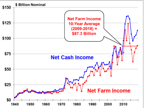
The August forecast of $88 billion is just above (+0.9%) the 10-year average of $87.3 billion and represents continued agriculture-sector economic weakness since 2013's record high of $123.7 billion.

Highlights

• Both net cash income and net farm income achieved record highs in 2013 but fell to recent lows in 2016 (Figure 1) before trending higher in each of the last three years 2017, 2018, and 2019.
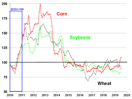
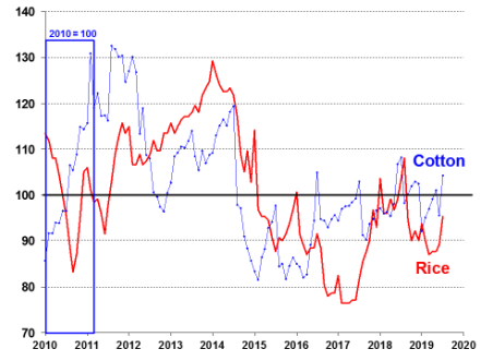
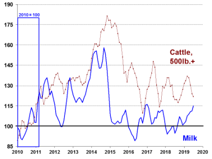
• Commodity prices (Figure A-1 to Figure A-4) have echoed the same pattern as farm income over the 2013-2019 period.
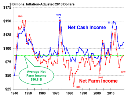
• When adjusted for inflation and represented in 2018 dollars (Figure 2), the net farm income for 2019 is projected to be on par with the average of $86.8 billion for net farm income since 1940.
• After declining for four consecutive years, total production expenses for 2019 (Figure 16), at $346.1 billion, are projected up slightly from 2018 (+0.4%), driven largely by higher costs for feed, labor, and property taxes.
• Global demand for U.S. agricultural exports (Figure 20) is projected at $134.5 billion in 2019, down from 2018 (-6.2%), due largely to a decline in sales to China.⁶
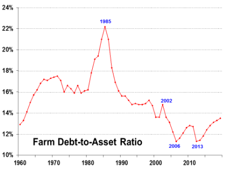
• Farm asset values and debt levels are projected to reach record levels in 2019—asset values at $3.1 trillion (+2.0%) and farm debt at $415.7 billion (+3.4%)—pushing the projected debt-to-asset ratio up to 13.5%, the highest level since 2003 (Figure 26).

Substantial Uncertainties Underpin the August 2019 Outlook

Abundant domestic and international supplies of grains and oilseeds suggest a fifth straight year of relatively weak commodity prices in 2019 (Figure A-1 through Figure A-4, and Table A-4). However, considerable uncertainty remains concerning the eventual outcome of the 2019 growing season and the prospects for improved market conditions heading into 2020.

As of early September, three major factors loom over U.S. agricultural markets and contribute to current uncertainty over both supply and demand prospects, as well as market prices:

• 1. First, wet spring conditions led to unusual plantings delays for the corn and soybean crops. This means that crop development is behind normal across much of the major growing regions and that eventual yields will depend on beneficial fall weather to achieve full crop maturity. Also, the late crop development renders crop growth vulnerable to an early freeze in the fall.
• 2. Second, large domestic supplies of corn, soybeans, wheat, and cotton were carried over into 2019 (Figure 6). Large corn and soybean stocks have kept pressure on commodity prices throughout the grain and feed complex in 2019.
• 3. Third, international trade disputes have led to declines in U.S. exports to China—a major market for U.S. agricultural products—and added to market uncertainty.⁷ In particular, the United States lost its preeminent market for soybeans—China. It is unclear how soon, if at all, the United States will achieve a resolution to its trade dispute with China or how international demand will evolve heading into 2020.

Figure 1. Annual U.S. Farm Sector Nominal Income, 1940-2019

Source: ERS, "2019 Farm Income Forecast," August 30, 2019. All values are nominal—that is, not adjusted for inflation. Values for 2019 are forecasts.

Figure 2. Annual U.S. Farm Sector Inflation-Adjusted Income, 1940-2019

Source: ERS, "2019 Farm Income Forecast," August 30, 2019. All values are adjusted for inflation using the chain-type GDP deflator, where 2018 = 100; Bureau of Economic Analysis, Real GDP Chained Dollars as of August 30, 2019. 2019 is forecast.

Late-Planted Corn and Soybean Crops Are Behind Normal Development

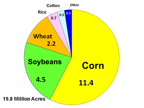
U.S. agricultural production activity got off to a very late start in 2019 due to prolonged cool, wet conditions throughout the major growing regions, particularly in states across the eastern Corn Belt. This resulted in record large prevented planting acres (Figure 3) and delays in the planting of the corn and soybean crops (Table 1), especially in Illinois, Michigan, Ohio, Wisconsin, and North and South Dakota.

As of August 22, 2019, U.S. farmers have reported to USDA that, of the cropland that they intended to plant this past spring, they were unable to plant 19.8 million acres due primarily to prolonged wet conditions that prevented field work. Such acres are referred to as "prevent plant (PPL)" acres. The previous record for total PPL acres was set in 2011 at 10.2 million acres. The 19.8 million PPL acres includes 11.4 million acres of corn and 4.5 million acres of soybeans—both establish new records by substantial margins. The previous record PPL for corn was 2.8 million acres in 2013, and for soybeans it was 2.1 million acres in 2015.

Figure 3. U.S. Farmers Report Record Acreage Prevented from Planting in 2019 (million acres)

Source: USDA, Farm Service Agency (FSA), FSA Crop Acreage Data Reported to FSA, 2019 Crop Year, as of August 22, 2019.

In addition, a sizeable portion of the U.S. corn and soybean crops were planted later than usual. Traditionally, 96% of the U.S. corn crop is planted by June 2, but in 2019 by that date only 67% of the crop had been planted (Table 1). Similarly, the U.S. soybean crop was planted with substantial delays. By June 16, only 67% of the U.S. soybean crop was planted, whereas an average of 93% of the crop has been planted by that date during the past five years.

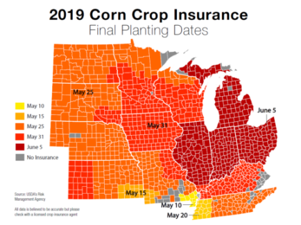
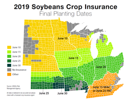
These planting delays have important implications for crop development as they push both crops' growing cycle into hotter, drier periods of the summer than usual and increase the risk of plant growth being shut off by an early freeze. But planting delays also increase the complexity of producer decisionmaking by pushing the planting date into the crop insurance "late planting period," when insurance coverage starts to decline with each successive day of delay (Figure 4).

When the planting occurs after the crop insurance policy's "final planting date," the "late planting period" comes into play. Producers must then decide whether to opt for "prevented planting" indemnity payments (valued at 35% of their crop insurance guarantee) or try to plant the crop under reduced insurance coverage with a heightened risk of reduced yields. Producer's choices were further complicated in 2019 by the Secretary of Agriculture's announcement on May 23 that only producers with planted acres would be eligible for "trade damage" assistance payments in 2019 under the Market Facilitation Program (MFP).⁸

Figure 4. Final Planting Dates (FPD) for Crop Insurance: Corn and Soybeans

Source: Farm Journal's AGPRO, "Is Prevent Plant the Most Profitable Option in 2019?," Sara Schafer, May 13, 2019, https://www.agprofessional.com/article/prevent-plant-most-profitable-option-2019. Notes: Acres planted on or before the FPD receive the full yield or revenue coverage that was purchased. If the crop is planted after the FPD, coverage is reduced by 1% per day throughout the late-planting period (25 days for both corn and soybeans). Policyholders who are prevented from planting some crop acres until after the FPD and choose to not plant the crop at all will receive 55% of the original guarantee for corn or 60% of the original guarantee for soybeans. For an additional premium, prevented planting coverage can be increased to 60% of the original coverage for corn acres or, for soybean acres, 65% of the original coverage. This choice must be made when the policy is purchased, however. A crop planted after the end of the late-planting period will be insured at the prevented-planting coverage level.

Figure 4. Final Planting Dates (FPD) for Crop Insurance: Corn and Soybeans

Source: Farm Journal's AGPRO, "Is Prevent Plant the Most Profitable Option in 2019?," Sara Schafer, May 13, 2019, https://www.agprofessional.com/article/prevent-plant-most-profitable-option-2019. Notes: Acres planted on or before the FPD receive the full yield or revenue coverage that was purchased. If the crop is planted after the FPD, coverage is reduced by 1% per day throughout the late-planting period (25 days for both corn and soybeans). Policyholders who are prevented from planting some crop acres until after the FPD and choose to not plant the crop at all will receive 55% of the original guarantee for corn or 60% of the original guarantee for soybeans. For an additional premium, prevented planting coverage can be increased to 60% of the original coverage for corn acres or, for soybean acres, 65% of the original coverage. This choice must be made when the policy is purchased, however. A crop planted after the end of the late-planting period will be insured at the prevented-planting coverage level.

Large Corn and Soybean Stocks Continue to Dominate Commodity Markets

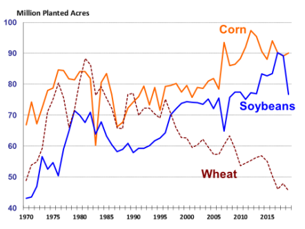
Corn and soybeans are the two largest U.S. commercial crops in terms of both value and acreage. For the past several years, U.S. corn and soybean crops have experienced strong growth in both productivity and output, thus helping to build stockpiles at the end of the marketing year. This has been particularly true for soybean production, which has seen rapid growth in yield, acres planted, and stocks. U.S. soybean production has been expanding rapidly since 1990, largely at the expense of the wheat sector which has been steadily losing acreage over the past several decades (Figure 5). This pattern reached a historic point in 2018 when, for the first time in history, U.S. soybean plantings (at 89.196 million acres) exceeded corn plantings (89.129 million acres).

The strong soybean plantings in 2018, coupled with the second-highest yields on record (51.6 bushels/acres), produced a record U.S. soybean harvest of 4.5 billion bushels and record ending stocks (1 billion bushels or a 27.2% stocks-to-use ratio) that year.⁹ However, the record soybean harvest in 2018, combined with the sudden loss of the Chinese soybean market (as discussed in the "Agricultural Trade Outlook" section of this report) discouraged many producers from planting soybeans in 2019. This contributed to a drop off (-14%) in soybean planted acres.

Figure 5. Planted Acres Since 1970: Corn, Soybeans, and Wheat

Source: NASS, August 12, 2019.

Most market watchers had expected to see a strong switch from soybean to corn acres in 2019 as a result of the record soybean stocks and weak prices related to the U.S.-China trade dispute. However, the wet spring made large corn plantings unlikely as corn yields tend to experience rapid deterioration when planted in June or later. Despite these indications, USDA's National Agricultural Statistics Service (NASS) released the results of its June acreage survey¹⁰ for corn planted acres at 91.7 million acres—well above market expectations. However, because the wet spring had caused widespread delayed planting, USDA announced that it would re-survey the 14 major corn-producing states. The updated survey results were released on August 12 and, at 90.0 million acres, confirmed higher-than-expected corn plantings.

As a result, the outlook for the U.S. corn crop has been pressured by the large planted acreage estimate but filled with uncertainty over the eventual success of the crop considering that it is being grown under unusually delayed conditions. Corn ending stocks are projected to surpass 2 billion bushels for the fourth consecutive year. Strong domestic demand from the livestock sector coupled with a robust export outlook are expected to support the season average farm price for corn at $3.60/bushel in the 2019/20 marketing year, unchanged from the previous year.

The outlook for the U.S. soybean crop is more certain: USDA projects a 19% drop in U.S. soybean production to 3.68 billion bushels. Despite the outlook for lower production in 2019, the record carry-over stocks from 2018, and the sudden loss of China as the principal buyer of U.S. soybeans in 2018, USDA projects lower soybean farm prices (-8%) at $8.40/bushel for the 2019/20 marketing year—the lowest farm price since 2006 (Figure 6).¹¹

Figure 6. Stocks-to-Use Ratios and Farm Prices: Corn, Soybeans, Wheat, and Cotton

Source: USDA, World Agricultural Outlook Board, World Agricultural Supply and Demand Estimates, August 12, 2019. All values are nominal. Values for 2019 are forecasts and are shown in dark blue. Notes: Stocks-to-use equals the ratio of season-ending stocks relative to the season's total usage.

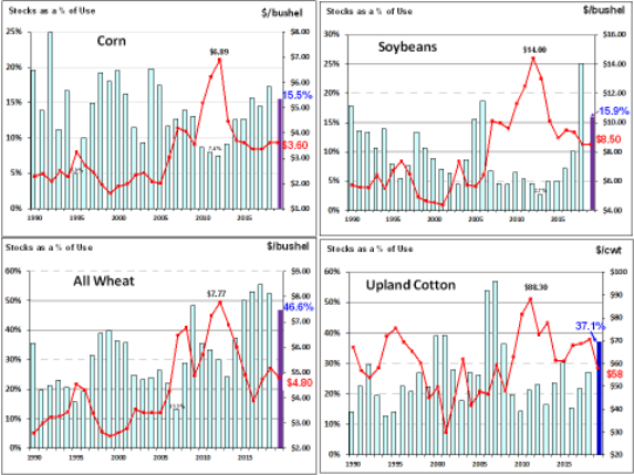
Both wheat and upland cotton farm prices for 2019 are projected down slightly from 2018—primarily due to the outlook for continued abundant stocks as indicated by the stocks-to-use ratios.

Diminished Trade Prospects Contribute to Market Uncertainty

The United States is traditionally one of the world's leading exporters of corn, soybeans, and soybean products—vegetable oil and meal. During the recent five-year period from 2013/2014 to 2017/2018, the United States exported 49% of its soybean production and 15% of its corn crop. As a result, the export outlook for these two crops is critical to both farm sector profitability and regional economic activity across large swaths of the United States as well as in international markets. However, the tariff-related trade dispute between the United States and China (as well as several major trading partners) has resulted in lower purchases of U.S. agricultural products by China in 2018 and 2019 and has cast uncertainty over the outlook for the U.S. agricultural sector, including the corn and soybean markets.¹²

Livestock Outlook for 2019 and 2020

Because the livestock sectors (particularly dairy and cattle, but hogs and poultry to a lesser degree) have longer biological lags and often require large capital investments up front, they are slower to adjust to changing market conditions than is the crop sector. As a result, USDA projects livestock and dairy production and prices an extra year into the future (compared with the crop sector) through 2020, and market participants consider this expanded outlook when deciding their market interactions—buy, sell, invest, etc.

Background on the U.S. Cattle-Beef Sector

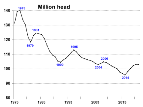
During the 2007-2014 period, high feed and forage prices plus widespread drought in the Southern Plains—the largest U.S. cattle production region—had resulted in an 8% contraction of the U.S. cattle inventory. Reduced beef supplies led to higher producer and consumer prices and record profitability among cow-calf producers in 2014. This was coupled with then-improved forage conditions, all of which helped to trigger the slow rebuilding phase in the cattle cycle that started in 2014 (Figure 7).

The expansion continued through 2018, despite weakening profitability, primarily due to the lag in the biological response to the strong market price signals of late 2014.¹³ The cattle expansion appears to have levelled off in 2019 with the estimated cattle and calf population unchanged from a year earlier at 103 million.¹⁴ Another factor working against continued expansion in cattle numbers is that producers are now producing more beef with fewer cattle.

Robust Production Growth Projected Across the Livestock Sector

Similar to the cattle sector, U.S. hog and poultry flocks have been growing in recent years and are expected to continue to expand in 2019.¹⁵ For 2019, USDA projects production of beef (+0.6%), pork (+5.0%), broilers (+1.7%), and eggs (+2.3%) to expand modestly heading into 2020. This growth in protein production is expected to be followed by continued positive growth rates in 2020: beef (+1.9%), pork (+2.8%), broilers (+1.1%), and eggs (+0.9%).

Figure 7. U.S. Beef Cattle Inventory (Including Calves) Since 1973

Source: NASS, Cattle, July 19, 2019. Notes: Inventory data are for July 1 of each year.

A key uncertainty for the meat-producing sector is whether demand will expand rapidly enough to absorb the continued growth in output or whether surplus production will begin to pressure prices lower. USDA projects that combined domestic and export demand for 2019 will continue to grow for red meat (+1.7%) and poultry (+1.5%) but at slightly slower rates than projected meat production, thus contributing to 2019's outlook for lower prices and profit margins for livestock.

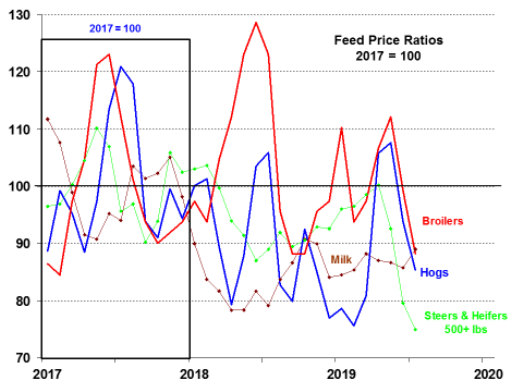
Livestock-Price-to-Feed-Cost Margins Signal Profitability Outlook

The changing conditions for the U.S. livestock sector may be tracked by the evolution of the ratios of livestock output prices to feed costs (Figure 8). A higher ratio suggests greater profitability for producers.¹⁶ The cattle-, hog-, and broiler-to-feed margins have all exhibited significant volatility during the 2017-2019 period.¹⁷ The hog, milk, and cattle feed ratios have trended downward during 2018 and 2019, suggesting eroding profitability. The broiler-to-feed price ratio has shown more volatility compared with the other livestock sectors but has trended upward from mid-2018 into 2019.

While this result varies widely across the United States, many small or marginally profitable cattle, hog, and milk producers face continued financial difficulties. Continued production growth of between 1% and 4% for red meat and poultry suggests that prices are vulnerable to weakness in demand. In addition, both U.S. and global milk production are projected to continue growing in 2019. As a result, milk prices could come under further pressure in 2019, although USDA is currently projecting milk prices up slightly in 2019.¹⁸ The lower price outlook for cattle, hogs, and poultry is expected to persist through 2019 before turning upward in 2020 (Table A-4).

Figure 8. Livestock Farm-Price-to-Feed Ratios, Indexed (Ratio of national average farm price per 100 lbs. of meat to per-unit feed cost. Indexed, 2017 = 100.)

Source: NASS, Agricultural Prices, August 30, 2019; calculations by CRS. Notes: The livestock feed price ratio is calculated as the farm price for milk, cattle (steers and heifers), hogs, and broilers to their major feed source: Cattle and hog feed cost is 100% corn; broilers feed cost is 58% corn and 42% soybeans; and dairy feed cost is a mix of corn, soybean meal, and alfalfa hay.

Gross Cash Income Highlights

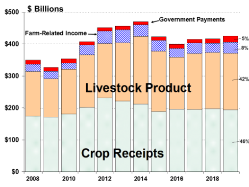
Projected farm-sector revenue sources in 2019 include crop revenues (46% of sector revenues), livestock receipts (42%), government payments (5%), and other farm-related income (8%), including crop insurance indemnities, machine hire, and custom work.¹⁹ Total farm sector gross cash income for 2019 is projected to be up (+2.2%) to $425.3 billion, driven by increases in both direct government payments (+42.5%) and other farm-related income (+19.3). Cash receipts from crop receipts (-1.7%) and livestock product (+0.5%) are down (-0.6%) in the aggregate (Figure 9).

Figure 9. Farm Cash Receipts by Source, 2008-2019

Source: ERS, "2019 Farm Income Forecast," August 30, 2019. All values are nominal—that is, not adjusted for inflation. Values for 2019 are forecasts. Percentage shares of gross farm income on the right-hand side are for 2019. Notes: Farm-related income includes income from custom work, machine hire, agro-tourism, forest product sales, crop insurance indemnities, and cooperative patronage dividend fees.

Crop Receipts

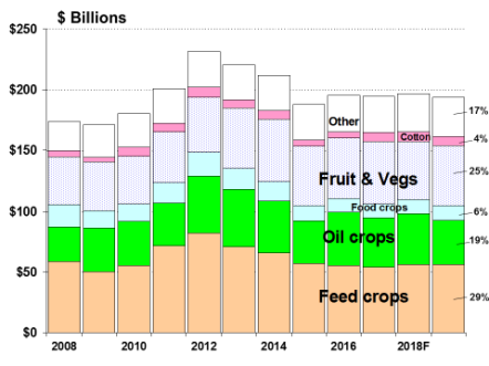
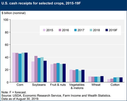
Total crop sales peaked in 2012 at $231.6 billion when a nationwide drought pushed commodity prices to record or near-record levels. In 2019, crop sales are projected at $193.7 billion, down 1.7% from 2018 (Figure 10). Projections for 2019 and percentage changes from 2018 include

• Feed crops—corn, barley, oats, sorghum, and hay: $56.3 billion (+0.4%);
• Oil crops—soybeans, peanuts, and other oilseeds: $36.3 billion (-14.0%);
• Fruits and nuts: $29.5 billion (+1.7%);
• Vegetables and melons: $19.6 billion (+6.0%);
• Food grains—wheat and rice: $12.3 billion (+6.5%);
• Cotton: $7.5 billion (-7.4%); and
• Other crops including tobacco, sugar, greenhouse, and nursery: $31.2 billion (+2.8%).

Figure 10. Crop Cash Receipts by Source, 2008-2019

Source: ERS, "2019 Farm Income Forecast," August 30, 2019. All values are nominal—that is, not adjusted for inflation. Values for 2019 are forecasts. Percentage shares of crop receipts on the right-hand side are for 2019.

Figure 11. Cash Receipts for Selected Crops, 2015-2019

Source: ERS, "2019 Farm Income Forecast," August 30, 2019. All values are nominal—that is, not adjusted for inflation. Values for 2019 are forecasts.

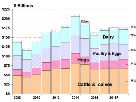
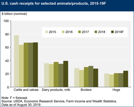
Livestock Receipts

The livestock sector includes cattle, hogs, sheep, poultry and eggs, dairy, and other minor activities. Cash receipts for the livestock sector grew steadily from 2009 to 2014, when it peaked at a record $212.3 billion. However, the sector turned downward in 2015 (-10.7%) and again in 2016 (-14.1%), driven largely by projected year-over-year price declines across major livestock categories (Table A-4 and Figure 12).

In 2017, livestock sector cash receipts recovered with year-to-year growth of 8.1% to $175.6 billion. In 2018, cash receipts increased slightly (+0.6%). In 2019, cash receipts are projected up 0.5% for the sector at $177.4 billion as cattle, hog, and dairy sales offset declines in poultry. Projections for 2019 (and percentage changes from 2018) include

• Cattle and calf sales: $67.3 billion (+0.3%);
• Poultry and egg sales: $38.9 billion (-15.8%);
• Dairy sales: valued at $39.7 billion (+12.7%);
• Hog sales: $24.5 billion (+16.2%); and
• Miscellaneous livestock:²⁰ valued at $7.0 billion (+2.1%).

Figure 12. U.S. Livestock Product Cash Receipts by Source, 2008-2019

Source: ERS, "2019 Farm Income Forecast," August 30, 2019. All values are nominal—that is, not adjusted for inflation. Values for 2019 are forecasts. Percentage shares of livestock receipts on the right-hand side are for 2019.

Figure 13. Cash Receipts for Selected Animal Products, 2015-2019

Source: ERS, "2019 Farm Income Forecast," August 30, 2019. All values are nominal—that is, not adjusted for inflation. Values for 2019 are forecasts.

Government Payments

Historically, government payments have included

• Direct payments (decoupled payments based on historical planted acres),
• Price-contingent payments (program outlays linked to market conditions),
• Conservation payments (including the Conservation Reserve Program and other environmental-based outlays),
• Ad hoc and emergency disaster assistance payments (including emergency supplemental crop and livestock disaster payments and market loss assistance payments for relief of low commodity prices), and
• Other miscellaneous outlays (including market facilitation payments, cotton ginning cost-share, biomass crop assistance program, peanut quota buyout, milk income loss, tobacco transition, and other miscellaneous payments).

Projected government payments of $19.5 billion in 2019 would be up 42.5% from 2018 and would be the largest taxpayer transfer to the agriculture sector (in absolute dollars) since 2005 (Figure 14 and Table A-4). The surge in federal subsidies is driven by large "trade-damage" payments made under the MFP initiated by USDA in response to the U.S.-China trade dispute.²¹ MFP payments (reported²² to be $10.7 billion) in 2019 include outlays from the 2018 MFP program that were not received by producers until 2019, as well as expected payments under the first and second tranches of the 2019 MFP program.²³

USDA ad hoc disaster assistance²⁴ is projected higher year-over-year at $1.7 billion (+87.1%). Payments under the Agricultural Risk Coverage and Price Loss Coverage programs are projected lower (-12.4%) in 2019 at a combined $2.8 billion compared with an estimated $3.2 billion in 2018 (see "Price Contingent" in Figure 14).²⁵

Figure 14. U.S. Government Farm Support, Direct Outlays, 1996-2019F

Source: ERS, "2019 Farm Income Forecast," August 30, 2019. All values are nominal—that is, not adjusted for inflation. Values for 2019 are forecasts. Percentage shares of government payments on the right-hand side are for 2019. Notes: Data are on a calendar-year basis and reflect the timing of the actual payment. "Direct Payments" include production flexibility contract payments enacted under the 1996 farm bill and fixed direct payments of the 2002 and 2008 farm bills. "Price-Contingent" outlays include loan deficiency payments, marketing loan gains, counter-cyclical payments, Average Crop Revenue Election, Price Loss Coverage, and Agricultural Risk Coverage payments. "Conservation" outlays include Conservation Reserve Program payments along with other conservation program outlays. "Ad Hoc and Emergency" includes emergency supplemental crop and livestock disaster payments and market loss assistance payments for relief of low commodity prices. "All Other" outlays include market facilitation payments, cotton ginning cost-share, biomass crop assistance program, peanut quota buyout, milk income loss, tobacco transition, and other miscellaneous payments.

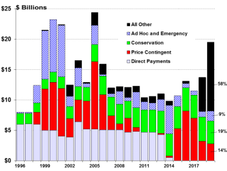
Conservation programs include all conservation programs operated by USDA's Farm Service Agency and the Natural Resources Conservation Service that provide direct payments to producers. Estimated conservation payments of $3.7 billion are forecast for 2019, down slightly (-8.4%) from $4.0 billion in 2018.

Total government payments of $19.5 billion represents a 5% share of projected gross cash income of $425.3 billion in 2019. In contrast, government payments are expected to represent 22% of the projected net farm income of $88.0 billion. The importance of government payments as a percentage of net farm income varies nationally by crop and livestock sector and by region.

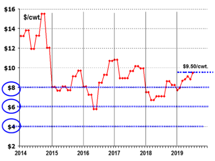
Dairy Margin Coverage Program Outlook

The 2018 farm bill (P.L. 115-334) made several changes to the previous Margin Protection Program (MPP), including a new name—the Dairy Margin Coverage (DMC) program—and expanded margin coverage choices from the original range of $4.00-$8.00 per hundredweight (cwt.).²⁶ Under the 2018 farm bill, milk producers have the option of covering the milk-to-feed margin at a $9.50/cwt. threshold on the first 5 million pounds of milk coverage under the program.

Figure 15. The Dairy Output-to-Input Margin Has Risen to $9.50/cwt. in Mid-2019 (The dairy margin equals the national average farm price of milk less average feed costs per 100 pounds.)

Source: NASS, Agricultural Prices, August 30, 2019; calculations by CRS. All values are nominal. Note: The margin equals the All Milk price minus a composite feed price based on the formula used by the DMC of the 2018 farm bill starting January 2019 and, for all prior months, the MPP of the 2014 farm bill (P.L. 113-79). See CRS Report R45525, The 2018 Farm Bill (P.L. 115-334): Summary and Side-by-Side Comparison.

The DMC margin differs from the USDA-reported milk-to-feed ratio shown in Figure 8 but reflects the same market forces. As of August 2019, the formula-based milk-to-feed margin used to determine government payments was at $9.45/cwt., just below the newly instituted $9.50/cwt. payment threshold (Figure 15), thus increasing the likelihood that DMC payments may be less available in the second half of 2019. In total, the DMC program is expected to make $600 million in payments in 2019, up from $250 million under the previous milk MPP in 2018.

Production Expenses

Total production expenses for 2019 for the U.S. agricultural sector are projected to be up slightly (+0.4%) from 2018 in nominal dollars at $346.1 billion (Figure 16). Production expenses peaked in both nominal and inflation-adjusted dollars in 2014, then declined for five consecutive years in inflation-adjusted dollars. However, in nominal dollars production expenses are projected to turn upward in 2019—the first upward turn since 2014.

Figure 16. Total Annual Farm Production Expenses, 1970-2019

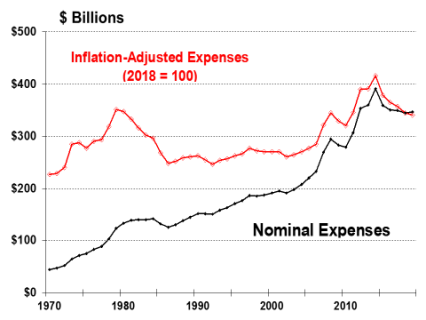Source: ERS, "2019 Farm Income Forecast," August 30, 2019. Nominal values are not adjusted for inflation. Inflation-adjusted expenses are calculated using the chain-type GDP deflator set to 2018 = 100. BEA, Real GDP Chained Dollars as of August 30, 2019. Amounts for 2019 are forecasts.

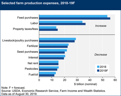
Production expenses affect crop and livestock farms differently. The principal expenses for livestock farms are feed costs, purchases of feeder animals and poultry, and hired labor. Feed costs, labor expenses, and property taxes are all projected up in 2019 (Figure 17). In contrast, fuel, land rent, interest costs, and fertilizer costs—all major crop production expenses—are projected lower.

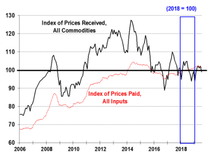
But how have production expenses moved relative to revenues? A comparison of the indexes of prices paid (an indicator of expenses) versus prices received (an indicator of revenues) reveals that the prices received index generally declined from 2014 through 2016, rebounded in 2017, then declined again in 2018 (Figure 18). Farm input prices (as reflected by the prices paid index) showed a similar pattern but with a smaller decline from their 2014 peak and have climbed steadily since mid-2016, suggesting that farm sector profit margins have been squeezed since 2016.

Figure 17. Farm Production Expenses for Selected Items, 2018 and 2019

Source: ERS, "2019 Farm Income Forecast," August 30, 2019. All values are nominal. Values for 2019 are forecasts.

Figure 18. Index of Monthly Prices Received vs. Prices Paid, 2006-2019

Source: NASS, Agricultural Prices, August 30, 2019. Calculations by CRS. Notes: Monthly farm prices for the 2010-2019 period have been divided by the annual average price for 2010 and multiplied by 100 such that 2015 = 100. Prices are indexed to 2015 = 100 to permit relative comparisons.

Cash Rental Rates

Renting or leasing land is a way for young or beginning farmers to enter agriculture without incurring debt associated with land purchases. It is also a means for existing farm operations to adjust production more quickly in response to changing market and production conditions while avoiding risks associated with land ownership. The share of rented farmland varies widely by region and production activity. However, for some farms it constitutes an important component of farm operating expenses. Since 2002, about 39% of agricultural land used in U.S. farming operations has been rented.²⁷

The majority of rented land in farms is rented from non-operating landlords. Nationally in 2017, 29% of all land in farms was rented from someone other than a farm operator. Some farmland is rented from other farm operations—nationally about 8% of all land in farms in 2017 (the most recent year for which data are available)—and thus constitutes a source of income for some operator landlords. Total net rent to non-operator landlords is projected to be down (-2.1%) to $12.5 billion in 2019.

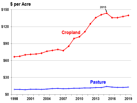
Average cash rental rates for 2019 were up (+1.4%) year-over-year ($140 per acre versus $138 in 2018). National average rental rates—which for 2019 were set the preceding fall of 2018 or in early spring of 2019—dipped in 2016 but still reflect the high crop prices and large net returns of the preceding several years, especially the 2011-2014 period (Figure 19). The national rental rate for cropland peaked at $144 per acre in 2015.²⁸

Figure 19. U.S. Average Farmland Cash Rental Rates Since 1998

Source: NASS, Agricultural Land Values, August 2019. All values are nominal.

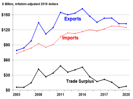
Agricultural Trade Outlook

U.S. agricultural exports have been a major contributor to farm income, especially since 2005. As a result, the financial success of the U.S. agricultural sector is strongly linked to international demand for U.S. products. Because of this strong linkage, the downturn in U.S. agricultural exports that started in 2015 (Figure 20) deepened the downturn in farm income that ran from 2013 through 2016 (Figure 1). Since 2018, the U.S. agricultural sector's trade outlook has been vulnerable to several international trade disputes, particularly the ongoing dispute between the United States and China.²⁹ A return to market-based farm income growth for the U.S. agricultural sector will likely necessitate improved international trade prospects.

Key U.S. Agricultural Trade Highlights

• USDA projects U.S. agricultural exports at $134.5 billion in FY2019, down (-6.2%) from $143.4 billion in FY2018. Export data include processed and unprocessed agricultural products. This downturn masks larger country-level changes that have occurred as a result of ongoing trade disputes (as discussed below).
• In FY2019, U.S. agricultural imports are projected up at $129.3 billion (1.4%), and the resultant agricultural trade surplus of $5.2 billion would be the lowest since 2006.

Figure 20. U.S. Agricultural Trade Since 2005 in 2018 Dollars

Source: ERS, Outlook for U.S. Agricultural Trade, August 29, 2019. Amounts for 2019 are projected.

• A substantial portion of the surge in U.S. agricultural exports that occurred between 2010 and 2014 was due to higher-priced grain and feed shipments, including record oilseed exports to China and growing animal product exports to East Asia. As commodity prices have leveled off, so too have export values (see the commodity price indexes in Figure A-1 and Figure A-2).
• In FY2017, the top three markets for U.S. agricultural exports were China, Canada, and Mexico, in that order. Together, these three countries accounted for 46% of total U.S. agricultural exports during the five-year period FY2014-FY2018 (Figure 21).
• However, in FY2019 the combined share of U.S. exports taken by China, Canada, and Mexico is projected down to 38% largely due to lower exports to China. The ordering of the top markets in 2019 is projected to be Canada, Mexico, the European Union (EU), Japan, and China, as China is projected to decline as a destination for U.S. agricultural exports.
• From FY2014 through FY2017, China imported an average of $26.2 billion of U.S. agricultural products. However, USDA forecasts China's imports of U.S. agricultural products to decline to $20.5 billion in FY2018 and to $10.9 billion in FY2019 as a result of the U.S.-China trade dispute.
• The fourth- and fifth-largest U.S. export markets have traditionally been the EU and Japan, which accounted for a combined 17% of U.S. agricultural exports during the FY2014-FY2018 period. These two markets have shown limited growth in recent years when compared with the rest of the world. However, their combined share is projected to grow to 19% in FY2019 (Figure 21).

Figure 21. U.S. Agricultural Export Value (Total and to China) Peaked in FY2014 (Inflation-adjusted using the implicit chain GDP deflator, 2018 = 100.)

Source: ERS, Outlook for U.S. Agricultural Trade, August 29, 2019. Amounts for 2019 are projected. All values are adjusted for inflation by CRS using the chain-type GDP deflator, where 2018 = 100; BEA, data as of August 30, 2019. Note: Data are for fiscal years (October to September).

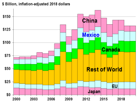
• The "Rest of World" (ROW) component of U.S. agricultural trade—South and Central America, the Middle East, Africa, and Southeast Asia—has shown strong import growth in recent years. ROW is expected to account for 43% of U.S. agricultural exports in FY2019. ROW import growth is being driven in part by both population and GDP growth but also from shifting trade patterns as some U.S. products previously targeting China have been diverted to new markets.
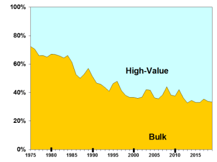
• Over the past four decades, U.S. agricultural exports have experienced fairly steady growth in shipments of high-value products—including horticultural products, livestock, poultry, and dairy. High-valued exports are forecast at $94.0 billion for a 69.9% share of U.S. agricultural exports in FY2019 (Figure 22).
• In contrast, bulk commodity shipments (primarily wheat, rice, feed grains, soybeans, cotton, and unmanufactured tobacco) are forecast at a record low 30.1% share of total U.S. agricultural exports in FY2019 at $40.5 billion. This compares with an average share of over 60% during the 1970s and into the 1980s. As grain and oilseed prices decline, so will the bulk value share of U.S. exports.

Figure 22. U.S. Agricultural Trade: Bulk vs. High-Value Shares

Source: ERS, Outlook for U.S. Agricultural Trade, AES-109, August 29, 2019. Amounts for 2019 are projected.

U.S. Farm and Manufactured Agricultural Product Export Shares

The share of agricultural production (based on value) sold outside the country indicates the level of U.S. agriculture's dependence on foreign markets, as well as the overall market for U.S. agricultural products.

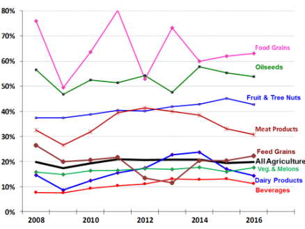
As a share of total farm and manufactured agricultural production, U.S. exports were estimated to account for 19.8% of the overall market for agricultural products from 2008 through 2016—the most recent data year for this calculation (Figure 23). The export share of agricultural production varies by product category:

• At the upper end of the range for export shares, the bulk food grain export share has varied between 50% and 80% since 2008, while the oilseed export share has ranged between 47% and 58%.
• The mid-spectrum range of export shares includes the export share for fruit and tree nuts, which has ranged from 37% to 45%, while meat products have ranged from 27% to 41%.
• At the low end of the spectrum, the export share of vegetable and melon sales has ranged from 15% to 18%, the dairy products export share from 9% to 24%, and the agricultural-based beverage export share between 7% and 13%.

Figure 23. U.S. Export Share of Farm and Manufactured Agricultural Production

Source: ERS, "U.S. Export Share of Production," as of February 9, 2018. Note: The export value share includes aggregated export values for all agricultural products—including bulk commodities and manufactured products—in the numerator and the total value of U.S. farm and manufactured agricultural production—estimated as farm cash receipts for crop and livestock production plus the value added by agricultural manufacturers—in the denominator.

Farm Asset Values and Debt

The U.S. farm income and asset-value situation and outlook suggest a relatively stable financial position heading into 2019 for the agriculture sector as a whole—but with considerable uncertainty regarding the downward outlook for prices and market conditions for the sector and an increasing dependency on international markets to absorb domestic surpluses and on federal support to offset lost trade opportunities due to ongoing trade disputes.

• Farm asset values—which reflect farm investors' and lenders' expectations about long-term profitability of farm sector investments—are projected to be up 2.0% in 2019 to a nominal $3.1 trillion (Table A-3). In inflation-adjusted terms (using 2018 dollars), farm asset values peaked in 2014 (Figure 24).

Figure 24. Real Estate Share Estimated at 83% of Total Farm Sector Assets in 2019

Source: ERS, "2019 Farm Income Forecast," August 30, 2019. All values are adjusted for inflation using the chain-type GDP deflator such that 2018 = 100; BEA, as of August 30, 2019. Data for 2019 are forecasts. Note: Nonreal-estate assets include financial assets, inventories of agricultural products, and the value of machinery and motor vehicles.

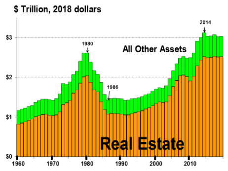
• Nominally higher farm asset values are expected in 2019 due to increases in both real estate values (+2.0%) and nonreal-estate values (+2.1%). Real estate is projected to account for 83% of total farm sector asset value.
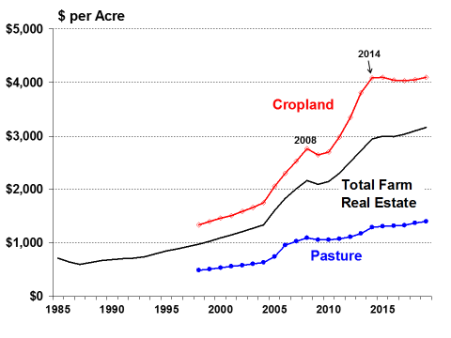
• Crop land values are closely linked to commodity prices. The leveling off of crop land values since 2015 reflects stagnant commodity prices (Figure 25). For 2019, USDA forecasts that prices for most major commodities will decline from 2018—wheat, barley, soybeans, cotton, choice steers, broilers, and eggs lower; sorghum, oats, rice, and pork products higher (Table A-4). However, these projections are subject to substantial uncertainty associated with international commodity markets.
• Total farm debt is forecast to rise to a record $415.7 billion in 2019 (+3.4%) (Table A-3). Farm equity—or net worth, defined as asset value minus debt—is projected to be up slightly (+1.8%) at $2.7 trillion in 2019 (Table A-3).
• The farm debt-to-asset ratio is forecast up in 2019 at 13.5%, the highest level since 2003 but still relatively low by historical standards (Figure 26).

Figure 25. U.S. Average Farm Land Values, 1985-2019

Source: NASS, Land Values 2019 Summary, August 2019. Notes: Farm real estate value measures the value of all land and buildings on farms. Separate cropland and pasture values are available only since 1998. All values are nominal.

Figure 26. U.S. Farm Debt-to-Asset Ratio, 1960-2019

Source: ERS, "2019 Farm Income Forecast," August 30, 2019. Values for 2019 are forecasts.

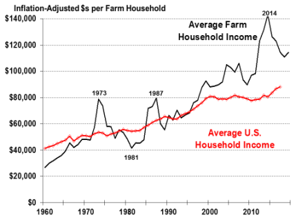
Average Farm Household Income

A farm can have both an on-farm and an off-farm component to its income statement and balance sheet of assets and debt.³¹ Thus, the well-being of farm operator households is not equivalent to the financial performance of the farm sector or of farm businesses because of the inclusion of nonfarm investments, jobs, and other links to the nonfarm economy.

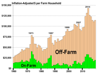
• Average farm household income (sum of on- and off-farm income) is projected at $116,060 in 2019 (Table A-2), up 4.7% from 2018 but 13.5% below the record of $134,165 in 2014.
• About 17% ($20,075) of total farm household income is from farm production activities, and the remaining 83% ($95,985) is earned off the farm (including financial investments).
• The share of farm income derived from off-farm sources had increased steadily for decades but peaked at about 95% in 2000 (Figure 27). Since 2014, over half of U.S. farm operations have had negative income from their agricultural operations.

Total vs. Farm Household Average Income

• Since the late 1990s, farm household incomes have surged ahead of average U.S. household incomes (Figure 28). In 2017 (the last year for which comparable data were available), the average farm household income of $111,744 was about 30% higher than the average U.S. household income of $86,220 (Table A-2).

Figure 27. U.S. Average Farm Household Income, by Source, 1960-2019

Source: ERS, "2019 Farm Income Forecast," August 30, 2019. All values are adjusted for inflation using the chain-type GDP deflator, 2018 = 100; BEA, data as of August 30, 2019. Values for 2019 are forecasts.

Figure 28. Farm Household Income Has Been Above U.S. Average Since 1996

Source: ERS, "2019 Farm Income Forecast," August 30, 2019. All values are adjusted for inflation using the chain-type GDP deflator, 2018 = 100; BEA, data as of August 30, 2019. Values for 2019 are forecasts.

Appendix. Supporting Charts and Tables

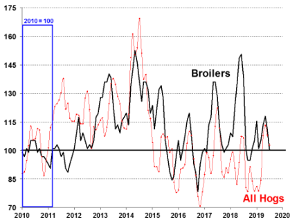
Figure A-1 to Figure A-4 present USDA data on monthly farm prices received for several major farm commodities—corn, soybeans, wheat, upland cotton, rice, milk, cattle, hogs, and chickens. The data are presented in an indexed format where monthly price data for year 2010 = 100 to facilitate comparisons.

USDA Farm Income Data Tables

Table A-1 to Table A-3 present aggregate farm income variables that summarize the financial situation of U.S. agriculture. In addition, Table A-4 presents the annual average farm price received for several major commodities, including the USDA forecast for the 2018-2019 marketing year.

Figure A-1. Monthly Farm Prices for Corn, Soybeans, and Wheat, Indexed Dollars

Source: NASS, Agricultural Prices, February 28, 2019. Calculations by CRS. Notes: Monthly farm prices for the 2010-2019 period have been divided by the annual average price for 2010 and multiplied by 100 such that 2010 = 100. Such price indexing facilitates relative comparisons.

Figure A-2. Monthly Farm Prices for Cotton and Rice, Indexed Dollars

Source: NASS, Agricultural Prices, February 28, 2019. Calculations by CRS. Notes: Monthly farm prices for the 2010-2019 period have been divided by the annual average price for 2010 and multiplied by 100 such that 2010 = 100. Such price indexing facilitates relative comparisons.

Figure A-3. Monthly Farm Prices for All-Milk and Cattle (500+ lbs.), Indexed Dollars

Source: NASS, Agricultural Prices February 28, 2019. Calculations by CRS. Notes: Monthly farm prices for the 2010-2019 period have been divided by the annual average price for 2010 and multiplied by 100 such that 2010 = 100. Such price indexing facilitates relative comparisons.

Figure A-4. Monthly Farm Prices for All Hogs and Broilers, Indexed Dollars

Source: NASS, Agricultural Prices, February 28, 2019. Calculations by CRS. Notes: Monthly farm prices for the 2010-2019 period have been divided by the annual average price for 2010 and multiplied by 100 such that 2010 = 100. Such price indexing facilitates relative comparisons.