Introduction
The U.S. farm sector is vast and varied. It encompasses production activities related to traditional field crops (such as corn, soybeans, wheat, and cotton) and livestock and poultry products (including meat, dairy, and eggs), as well as fruits, tree nuts, and vegetables. In addition, U.S. agricultural output includes greenhouse and nursery products, forest products, custom work, machine hire, and other farm-related activities. The intensity and economic importance of each of these activities, as well as their underlying market structure and production processes, vary regionally based on the agro-climatic setting, market conditions, and other factors. As a result, farm income and rural economic conditions may vary substantially across the United States.1 However, this report focuses singularly on aggregate national net farm income and the status of the farm debt-to-asset ratio as reported by the U.S. Department of Agriculture's (USDA's) Economic Research Service (ERS).2
Annual U.S. net farm income is the single most watched indicator of farm sector well-being, as it captures and reflects the entirety of economic activity across the range of production processes, input expenses, and marketing conditions that have prevailed during a specific time period. When national net farm income is reported together with a measure of the national farm debt-to-asset ratio, the two summary statistics provide a quick and widely referenced indicator of the economic well-being of the national farm economy.
|
Measuring Farm Profitability Two different indicators measure farm profitability: net cash income and net farm income. Net cash income compares cash receipts to cash expenses. As such, it is a cash flow measure representing the funds that are available to farm operators to meet family living expenses and make debt payments. For example, crops that are produced and harvested but kept in on-farm storage are not counted in net cash income. Farm output must be sold before it is counted as part of the household's cash flow. Net farm income is a more comprehensive measure of farm profitability. It measures value of production indicating the farm operator's share of the net value added to the national economy within a calendar year, independent of whether it is received in cash or noncash form. As a result, net farm income includes the value of home consumption, changes in inventories, capital replacement, and implicit rent and expenses related to the farm operator's dwelling that are not reflected in cash transactions. Thus, once a crop is grown and harvested it is included in the farm's net income calculation, even if it remains in on-farm storage. Key Concepts
|
USDA's 2017 Farm Income Forecast
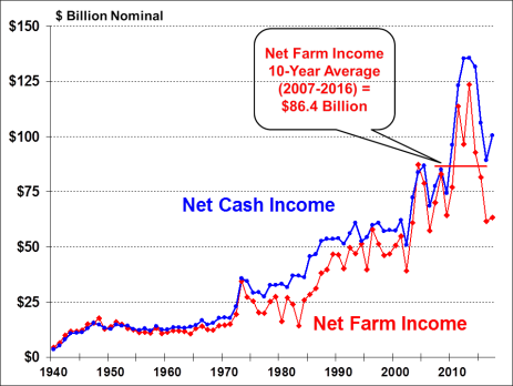
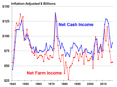
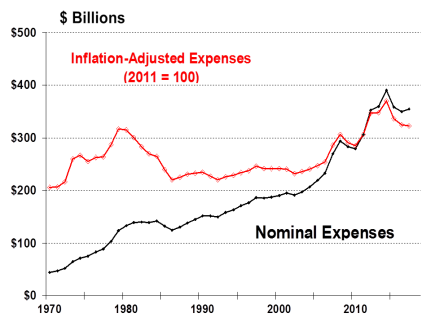
According to ERS, net farm income is forecast at $63.4 billion in 2017, up 3% from last year (Table 1).3 The forecast rise in 2017 net farm income comes after three consecutive years of decline from 2013's record high of $123.8 billion. The 2017 net farm income forecast is substantially below the 10-year average of $86.4 billion (Figure 1). In inflation-adjusted dollars, the 2017 forecast is the second lowest since 2003 (Figure 2). Net cash income is also projected to be up in 2017 but by a larger share (12.5%), driven largely by sales from previous years' inventory, to $100.4 billion. Since the record highs of 2013, net farm income and net cash income have fallen by 49% and 26%, respectively (Figure 1).
Selected Highlights
- After three consecutive years of decline, net cash income and net farm income are both forecast to rise in 2017 relative to 2016. The downward trend in farm income since 2013 was primarily a result of the significant decline in most farm commodity prices since the 2013-2014 period.
- Farm prices for most feedstuffs—feed grains, hay, and wheat—declined during both 2015/16 and 2016/17 as U.S. and global grain stocks rebuild (Table 4 and Figure 28 to Figure 31). In contrast, cotton and soybean prices showed resilience in 2016. The price outlook for 2017 is mixed.
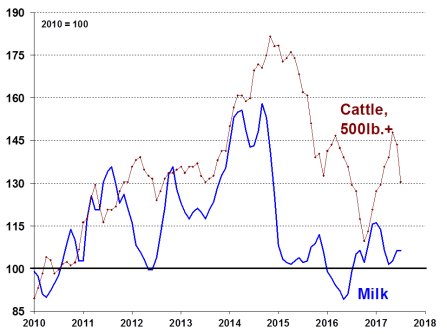
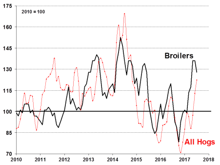
- Poultry, hog, and milk prices are all projected to be higher in 2017, albeit well below their market highs of 2014/15 (Table 4 and Figure 32 to Figure 35). Cattle prices are projected to be down slightly in 2017.
- Government payments in 2017 are projected to be down slightly (-0.2%) to $13.0 billion (Figure 13). Lower marketing-assistance loan benefits and the end of the cotton ginning cost-share program, which paid $326 million in 2016, more than offset projected higher Price Loss Coverage (PLC) and Agriculture Risk Coverage (ARC) program payments of $8.4 billion—triggered by lower commodity prices. Outlays under the ARC and PLC programs (which are contingent on market prices) are intended to provide some relief for participating producers from the market downturn.
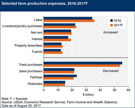
- Total production expenses (Figure 14), at $355.1 billion, are projected to be up 1.3% in 2017, driven largely by replacement animal, labor, and interest costs.
- U.S. farm prices are supported in part by global demand for U.S. agricultural exports (Figure 18), which are expected to rise to $139.8 billion (+8%) in 2017—still well below the record of $152.3 billion set in 2014.4
- Farm asset values are projected to be up, at $3,075 billion (+4%) in 2017, as land values strengthen. A rise in farm debt to $390 billion (+4.4%) is expected to result in a rise in the debt-to-asset ratio to 12.7%, the highest level since 2011 (Figure 24).
|
Figure 2. Annual U.S. Farm Sector Inflation-Adjusted Income, 1940 to 2017F |
 |
|
Source: ERS, "2017 Farm Income Forecast," August 30, 2017. All values are adjusted for inflation using the chain-type gross domestic product (GDP) deflator, where 2009 = 100, Office of Management and Budget (OMB), Historical Tables, Table 10.1, https://www.whitehouse.gov/omb/budget/Historicals; 2017 is forecast. |
Overview of U.S. Agriculture in 2017
Crop Outlook
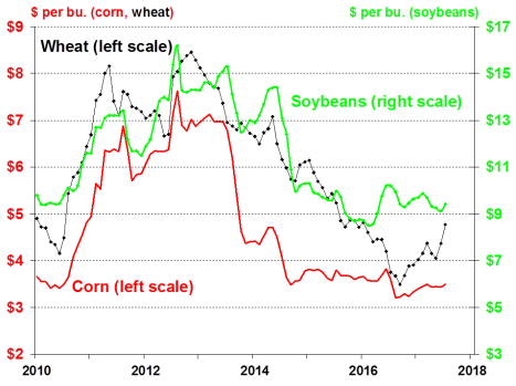
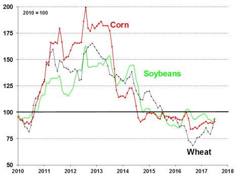
Normal weather conditions prevailed in most U.S. growing regions, with the notable exception of Montana and the Dakotas, where severe drought impacted the small-grain crops. The north-central drought expanded in late summer into Idaho, Oregon, and Washington and parts of southern Iowa. As a result of the north-central drought, USDA is forecasting substantially lower yield and output for spring-grown barley and wheat crops in the affected states. Overall, 2017 U.S. wheat production is estimated to be down nearly 25% from last year. This production shortfall, coupled with continued strong export demand for U.S. wheat, is behind an 18% increase in the U.S. wheat farm price during the 2017/18 crop year to $4.60 per bushel—still below the $7.77 achieved in 2012 (Figure 28). Reduced rainfall also appears to have lowered sorghum, oat, and forage-crop prospects in affected regions. However, the effect on the corn and soybean crops appears minimal.
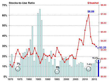
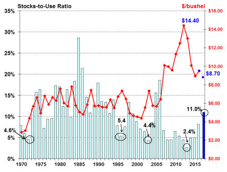
Corn and soybeans are the two largest U.S. commercial crops in terms of both value and quantity. These crops provide important inputs for the domestic livestock, poultry, and biofuels sectors. In addition, the United States is traditionally one of the world's leading exporters of corn, soybeans, and soybean products—vegetable oil and meal. As a result, the outlook for these two crops is critical to both farm sector profitability and regional economic activity across large swaths of the United States as well as in international markets. For the past several years, U.S. corn and soybean crops have experienced remarkable growth in both productivity and output. Both crops had record harvests in 2014, above-average harvests in 2015, and record harvests again in 2016, thus helping to build stockpiles at the end of the marketing year (Figure 3 and Figure 4) and pressure prices lower in U.S. and international markets (Figure 28 through Figure 31) in 2017.
Planted acres for both feed grains (101.8 million acres) and wheat (45.7 million acres) were down in 2017 by 6.4% and 9.0%, respectively, from 2016. However, soybean-planted acres were estimated at a record 89.5 million (+7.3%). The 2017 yield outlook for both corn and soybean crops is above trend (although down from the previous year's record highs) for both, with expectations for the second-highest soybean yield (49.4 bu./ac.) and third-highest corn yield (169.9 bu./ac.) on record. The record soybean plantings coupled with the strong yield outlook combine for an expected record large soybean harvest of 4.4 billion bushels in 2017. As a result of the expected record harvest, soybean prices are projected to be lower (-3.2%) at $9.20 per bushel. Despite lower area, yield, and production, U.S. corn supplies are expected to continue to build in 2017, thus pushing the expected crop-year price down 4.5% to $3.20/bu. The corn and soybean price forecasts for 2017 are the lowest since the 2006 crop year for both crops.
The length and severity of the California drought has important national implications for retail food prices. California production accounts for about one-third of U.S. vegetables, almost two-thirds of U.S. fruit and nuts, about 20% of U.S. milk, and a substantial portion of wine.5 Abundant precipitation during the 2016/17 winter has alleviated drought conditions in much of the northern portion of the state. However, the drought, which began in 2012, persists in the lower third of the state.6
The effects of hurricanes Harvey and Irma on U.S. agriculture are still being ascertained but have likely resulted in extensive crop damage. Harvey's impact focused on Texas and Louisiana. (Affected crops include upland cotton, rice, soybeans, sugar, and others.) Irma's impact focused on Florida, Georgia, South Carolina, and Alabama. (Affected crops include citrus, sugar, peanuts, upland cotton, soybeans, and specialty crops.) USDA's National Agricultural Statistics Service (NASS) announced on September 12, 2017, that it would collect harvested acreage information for a number of crops in affected states in preparation for the October Crop Production report.7 These additional data will help to better assess the full impact.
Livestock Outlook
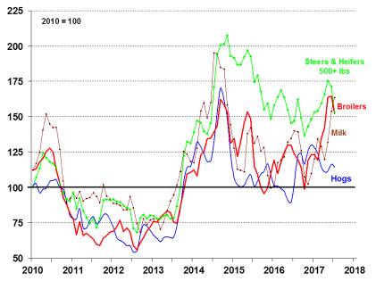
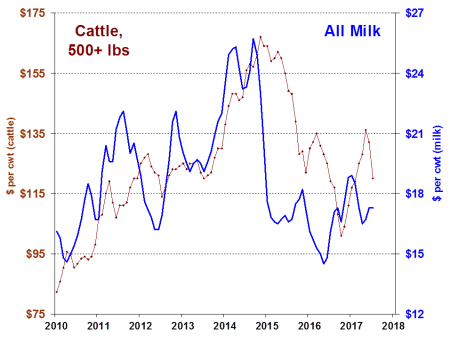
The changing conditions for the U.S. livestock sector may be tracked by the evolution of the ratios of livestock output prices to feed costs (Figure 5). A higher ratio suggests greater profitability for producers.8 The cattle-, hog-, and broiler-to-feed margins all moved upwards in the first half of 2017.9 The hog sector, despite seeing its hog-to-feed ratio dip lower in early 2017, remains profitable. However, continued strong production growth of between 2% and 3% for red meat and poultry suggests that prices are vulnerable to any weakness in demand.
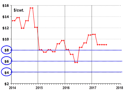
Milk prices and the milk-to-feed ratio turned sharply higher in 2017, suggesting improving profitability. However, this result varies widely across the United States with many small or marginally profitable producers facing continued financial difficulties. In addition, both U.S. and global milk production are projected to continue growing through 2017. As a result, milk prices could come under further pressure in the last half of 2017. With respect to the federal milk margin protection program (MPP) instituted by the 2014 farm bill (Agricultural Act of 2014, P.L. 113-79), the formula-based milk-to-feed margin used to determine government payments is likely to remain above the $8.00 per hundredweight (cwt.) threshold needed to trigger payments (Figure 6).10 The MPP margin differs from the USDA-reported milk-to-feed ratio shown in Figure 5 but reflects the same market forces.
|
Figure 6. The MPP Margin Projected to Remain Above $8/cwt. in 2017 (National average farm price of milk less average feed costs per 100 lbs.) |
 |
|
Source: USDA, NASS, Agricultural Prices, August 30, 2017; calculations by CRS. All values are nominal. Note: Based on the feed price formula used by the Margin Protection Program of the 2014 farm bill (P.L. 113-79); see CRS Report R43465, Dairy Provisions in the 2014 Farm Bill (P.L. 113-79), by [author name scrubbed]. |
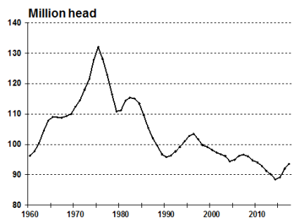
Similarly, U.S. hog and cattle herds and poultry flocks are expected to continue to expand into 2018.11 Cattle and hog expansion is primarily the result of a substantial lag in the biological response to the strong market price signals of late 2014. The U.S. cattle sector has been expanding since 2014. During the 2007 to 2014 period, high feed and forage prices, plus widespread drought in the Southern Plains—the largest U.S. cattle production region—had resulted in an 8% contraction of the U.S. cattle inventory (Figure 7). Reduced beef supplies led to higher producer and consumer prices, which in turn triggered the slow rebuilding phase in the cattle cycle that started in 2014 (see the price-to-feed ratio for steers and heifers, Figure 5). The resulting continued expansion of beef supplies pressured market prices lower into 2017. However, projections of expanding domestic and international demand across all meat categories through 2018 is expected to largely stem the decline in prices and profitability in 2017 (Figure 32).
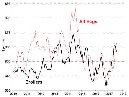
In 2014, the U.S. hog sector was hit by the rapid outbreak and spread of the porcine epidemic diarrhea virus (PEDv), which caused market worries about reduced U.S. pork production. The incidence of PEDv since the winter of 2014/15 has declined, and initial market fears have subsided. However, the related 2014 surge in hog prices elicited substantial producer response, and the resulting continued expansion of pork supplies through 2016 has weighed on market prices (Figure 34). For pork, as with beef and poultry, projections of expanding domestic and international demand have supported prices and profitability in 2017.
|
Figure 7. The U.S. Beef Cattle Inventory (Including Calves) Since 1960 |
 |
|
Source: USDA, NASS, Cattle, January 31, 2017. Notes: Inventory data are for January 1 of each year. |
During spring 2015, the U.S. poultry industry experienced a severe outbreak of highly pathogenic avian influenza.12 The outbreak ended by early summer 2015. More than 48 million chickens, turkeys, and other poultry were euthanized to stem the spread of the disease. Turkey and egg-laying hen farms in Minnesota and Iowa were the hardest hit. Commercial broiler farms were not affected. USDA estimates that egg production declined over 5% in 2015, pushing egg prices up 28% that year. The recovery in broiler and egg production was swift as prices fell 7% and 53% in 2016, respectively. In 2017, strong domestic and export demand is expected to push prices up by a projected 11.5% and 2.7% for broilers and eggs.
In sum, production of beef (+5.3%), pork (+2.2%), broilers (+1.5%), and eggs (+2.3%) are projected to expand relatively robustly in 2017. Meat and egg supplies are projected to continue growing in 2018 at 1.4% to 3.4%, respectively. Fortunately for producers, USDA projects that combined domestic and export demand will grow by 2.2% in 2018, thus helping to support red meat, poultry, and egg prices and profit margins in 2017 (Table 4).
Gross Cash Income Highlights
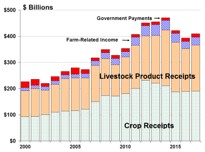
Total farm sector gross cash income for 2017 is projected to be up (+4%), to $409.4 billion, driven by a $14.1 billion (4%) increase in the value of agricultural sector production. That is nevertheless well below 2014's record $470.6 billion (Figure 8). The projected 2017 increase includes higher livestock returns (+8.4%) and farm-related income (+7%). Record yields helped to offset lower crop prices, leaving total crop revenues up slightly (0.3%), at $190.1 billion in 2017. Similarly, larger animal product output and improving prices (for hogs, broilers, eggs, and milk) are expected to push livestock cash receipts higher, to $176.5 billion. Farm-sector revenue sources and shares include crop revenues (46% of sector revenues), livestock receipts (43%), government payments (3%), and other farm-related income, including crop insurance indemnities, machine hire, and custom work (7%).
 |
|
Source: ERS, "2017 Farm Income Forecast," August 30, 2017. All values are nominal, that is, not adjusted for inflation. 2017 is a forecast. Notes: Receipts from crop and livestock product sales, and government payments, are described in more detail below. Farm-related income includes income from custom work, machine hire, agrotourism, forest product sales, insurance indemnities, and cooperative patronage dividend fees. |
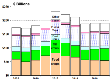
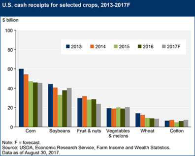
Crop Receipts
Total crop sales peaked in 2012 at a record $231.6 billion when a nationwide drought pushed commodity prices to record or near-record levels. In 2017, crop sales are projected at $190.1 billion, up slightly from 2016, as record yields offset lower prices for corn, soybeans, and cotton (Figure 9). The crop sector includes 2017 projections (and percentage changes from 2016) for:
- feed crops—corn, barley, oats, sorghum, and hay—of $54.6 billion (-0.4%);
- oil crops—soybeans, peanuts, and other oilseeds—of $42.6 billion (+5.8%);
- food grains—wheat and rice—of $11.0 billion (-3.0%);
- fruits and nuts of $23.8 billion (-17.2%);
- vegetables and melons of $20.4 billion (+6.8%);
- cotton of $7.4 billion (+25.6%); and
- all other crops—including tobacco, sugar, greenhouse, and nursery crops—of $28.4 billion (+1.2%).
 |
|
Source: ERS, "2017 Farm Income Forecast," August 30, 2017. All values are nominal, that is, not adjusted for inflation. 2017 is a forecast. |
 |
|
Source: ERS, "2017 Farm Income Forecast," August 30, 2017. All values are nominal, that is, not adjusted for inflation. 2017 is a forecast. |
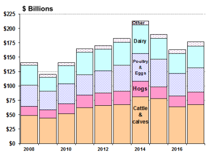
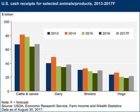
Livestock Receipts
The livestock sector includes cattle, hogs, sheep, poultry and eggs, dairy, and other minor activities. Cash receipts for the livestock sector grew steadily following the severe downturn of 2009, peaking in 2014 at a record $212.8 billion. However, the sector turned downward in 2015 (-10.8%) and again in 2016 (-12.3%)—driven largely by projected year-over-year price declines across major livestock categories (Table 4 and Figure 11). In 2017, livestock sector cash receipts are projected to show some recovery, with year-to-year growth of 8.4%, to $176.5 billion. Highlights include 2017 projections (and percentage changes from 2016) for
- cattle and calf sales of $67.6 billion (5.7%),
- hog sales of $21.6 billion (14.6%),
- poultry and egg sales of $41.9 billion (+8.4%), and
- dairy sales, valued at $38.4 billion (+11.1%).
Government Payments
Government payments in 2017 are projected to be down slightly, by 0.2% from 2016, at $13.0 billion. Declining farm prices are expected to trigger substantial payments under the price-contingent programs—the PLC and ARC programs (Figure 13). However, increases in ARC and PLC payments are expected to be offset by declines in marketing-assistance loan benefits and the end of the one-time cotton ginning cost-share program (included in "All Other"), which made $326 million in payments in 2016.
ARC and PLC are new revenue support programs established by the 2014 farm bill (Agricultural Act of 2014; P.L. 113-79).13 The PLC program replaced the previous Counter-Cyclical Price (CCP) program, but with a set of reference prices based on substantially higher support levels for most program crops. ARC relies on a five-year moving average price trigger in its payment calculation but also adopts the PLC reference price as the minimum guarantee in years when market prices fall below it. These higher relative support levels are expected to trigger payments of $8.4 billion in 2017, up from $8.2 billion in 2016.
Government payments of $13 billion would represent a relatively small share (3%) of projected gross cash income of $409.4 billion in 2017. In contrast, government payments are expected to represent 20% of net farm income of $63.4 billion in 2017 (Table 1). However, the importance of government payments as a percent of net farm income varies nationally by crop and livestock sector and by region.
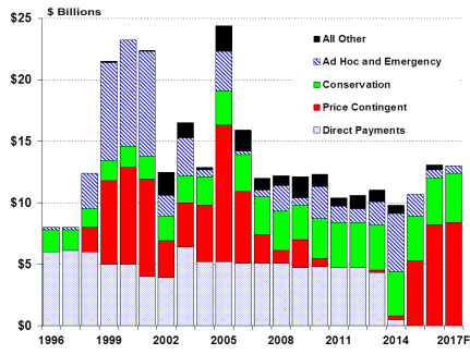
Payments under the price-contingent marketing loan benefit are forecast at $11 million in 2017, down sharply from $206 million in 2016, as program crop prices are expected to remain above most program loan rates through 2017 (Table 4). Farm fixed direct payments, whose decoupled payment rates were fixed in previous legislation, were eliminated by the 2014 farm bill.14 The Margin Protection Program (MPP) for dairy is expected to earn savings as producer premiums paid exceed federal MPP payments by $5 million in 2017.
Conservation programs include all conservation programs operated by USDA's Farm Service Agency (FSA) and the Natural Resources Conservation Service (NRCS) that provide direct payments to producers. Estimated conservation payments of $4.0 billion are forecast for 2017, up 6% from 2016.
Supplemental and ad-hoc disaster assistance payments are forecast at $559 million in 2017, a 15% decline from $658 million in 2016. The decline is largely due to an expected decline in outlays under the Livestock Indemnity and Livestock Forage Programs.15
Production Expenses
Total production expenses for 2017 for the U.S. agricultural sector are projected to be up 1.3% in nominal dollars, at $355 billion (Figure 14) following two years of decline. Multi-year reductions in farm production expenses are relatively rare, the most recent occurrence being 1984 to 1986. Changes in input prices (i.e., expenses) typically lag commodity price changes.
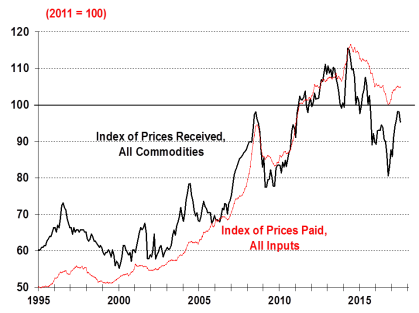
Commodity prices received by farmers generally declined from 2014 through 2016 before rebounding in 2017 (Figure 15). Farm input prices showed a similar pattern but with a much smaller decline from their 2014 peak, thus putting pressure on producer margins in recent years.
Production expenses will affect crop and livestock farms differently. The principal expenses for livestock farms are feed costs and purchases of feeder animals and poultry. Feed costs are projected to be down in 2017 (-2.9%), while replacement animal costs have increased by 3% (Figure 16). Taken together, the principal livestock expenses are forecast to be down 1.2% from 2016, at $77.1 billion.
The principal crop expenses—including fertilizers, pesticides, feed, and seed—are forecast to be down by about 3%, to $91.8 billion. Miscellaneous operating expenses, which are projected to be unchanged at $36.6 billion, include crop insurance premiums and thus directly impact crop production. Total farm production expenses were up largely because of higher interest charges, hired labor costs, net rent, and miscellaneous expenses that are not attributed to a particular production activity.
 |
|
Source: ERS, "2017 Farm Income Forecast," August 30, 2017. Inflation-adjusted expenses are calculated using the chain-type GDP deflator, OMB, Historical Tables, Table 10.1. Amounts for 2017 are forecasts. |
Cash Rental Rates
Renting or leasing land is a way for young or beginning farmers to enter agriculture without incurring debt associated with land purchases. It is also a means for existing farm operations to adjust production more quickly in response to changing market and production conditions while avoiding risks associated with land ownership.
The share of rented farmland varies widely by region and production activity. However, for some farms it constitutes an important component of farm operating expenses. Since 2002, about 38% of agricultural land used in U.S. farming operations has been rented.16
Some farmland is rented from other farm operations—nationally about 8% of all land in farms in 2012 (the most recent year for which data are available)—and thus constitutes a source of income for some operator landlords. However, the majority of rented land in farms is rented from non-operating landlords. Nationally in 2012, 30% of all land in farms was rented from someone other than a farm operator. Total net rent to non-operator landlords is projected to be up by 1.4%, at $15.1 billion in 2017.
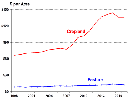
Average cash rental rates for 2017—which were set the preceding fall of 2016 or in early spring of 2017—still reflect the high crop prices and large net returns of the preceding several years (especially the 2011 to 2014 period) and have yet to decline substantially (Figure 17). The national rental rate for crop land peaked at $144 per acre in 2015 and has been at $136 per acre for the past two years (2016 and 2017).
|
Figure 17. U.S. Average Farm Land Cash Rental Rates Since 1998 |
 |
|
Source: NASS, "Quick Stats," downloaded August 30, 2017. All values are nominal. |
Agricultural Trade Outlook
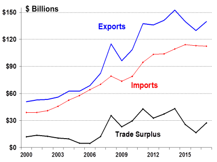
U.S. agricultural exports have been a major contributor to farm income, especially since 2005. As a result, the sharp downturn in those exports that followed 2014's peak of $152.3 billion both coincided with and deepened the downturn in farm income that started in 2015.
USDA projects U.S. agricultural exports at $139.8 billion in 2017, up 8% from 2016's total (Figure 18), due largely to an improving economic outlook in several major foreign importing countries. USDA also projects that U.S. agricultural imports will be higher, at $116.2 billion (+3%), with a resulting agricultural trade surplus of $23.6 billion (+42%).
|
Figure 18. U.S. Agricultural Trade Since 2000, Nominal Values |
 |
|
Source: ERS, Outlook for U.S. Agricultural Trade, AES-101, August 29, 2017; 2017 is a projection. |
Key U.S. Agricultural Trade Highlights
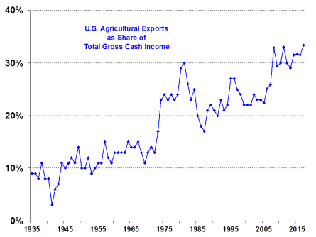
- As a share of total gross farm receipts, U.S. agricultural exports are projected to account for 33.4% of gross cash earnings in 2017 (Figure 19).
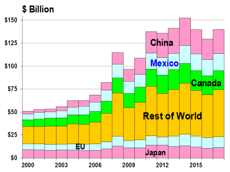
- The top three markets for U.S. agricultural exports are China, Canada, and Mexico, in that order. Together, these three countries are expected to account for $65.6 billion, or 47% of total U.S. agricultural exports in FY2017 (Figure 20).
- A substantial portion of the increase in U.S. agricultural exports since 2010 has also been due to higher-priced grain and feed shipments, plus record oilseed exports to China and growing animal product exports to East Asia.
- The fourth- and fifth-largest U.S. export markets are the European Union (EU) and Japan, which are projected to account for a combined 17% of U.S. agricultural exports in FY2017. However, these two markets have shown relatively limited growth in recent years when compared with the rest of the world.
|
Figure 19. U.S. Agricultural Export Value as Share of Gross Cash Income |
 |
|
Source: ERS, Outlook for U.S. Agricultural Trade, AES-101, August 29, 2017. Amount for 2017 is a projection. |
|
Figure 20. U.S. Agricultural Exports Have Leveled Off Since 2011 |
 |
|
Source: ERS, Outlook for U.S. Agricultural Trade, AES-101, August 29, 2017. Amounts for 2017 are projected. |
- The "Rest of World" (ROW) component of U.S. agricultural trade—the Middle East, Africa, and Southeast Asia—has shown strong import growth in recent years. ROW is expected to account for 36% of U.S. agricultural exports in 2017.
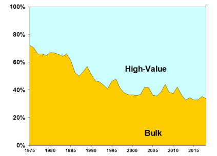
- Over the past four decades, U.S. agricultural exports have experienced fairly steady growth in shipments of high-value products (Figure 21). As grain and oilseed prices decline, so will the bulk value share of U.S. exports.
- Bulk commodity shipments (primarily wheat, rice, feed grains, soybeans, cotton, and unmanufactured tobacco) are forecast at a 35% share of total U.S. agricultural exports in 2017, at $49.3 billion. This compares with an average share of over 60% during the 1970s and 1980s.
- In contrast, high-valued export products—including horticultural products, livestock, poultry, and dairy—are forecast at $90.5 billion for a 66.4% share of U.S. agricultural exports in 2017.
|
Figure 21. U.S. Agricultural Trade: Bulk vs. High-Value Shares |
 |
|
Source: ERS, Outlook for U.S. Agricultural Trade, AES-101, August 29, 2017. Percentage for 2017 is a projection. |
Farm Asset Values and Debt
The U.S. farm income and asset-value situation and outlook suggest a relatively stable financial position heading into 2017 for the agriculture sector as a whole but with considerable uncertainty regarding the downward outlook for prices and market conditions for the sector and an increasing dependency on international markets to absorb domestic surpluses:
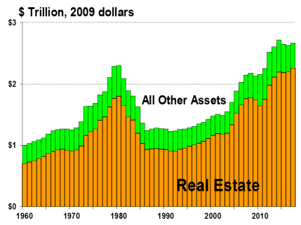
- Farm asset values—which reflect farm investors' and lenders' expectations about long-term profitability of farm sector investments—are projected to be up 4% in 2017 to a nominal $3,075 billion (Table 3). In inflation-adjusted terms (using 2009 dollars), farm asset values peaked in 2014 (Figure 22).
- Higher farm asset values are expected in 2017 due to strength in real estate values (+4.6%) that more than offsets a decline in non-real-estate values (-5.1%). Real estate traditionally accounts for the bulk of total value of farm sector assets—nearly an 81% share.
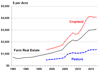
- Crop land values are closely linked to commodity prices. The leveling off of crop land values in 2017 reflects mixed forecasts for commodity prices (corn, soybeans, and cotton lower; wheat, rice, and livestock products higher) and the uncertainty associated with international commodity markets (Figure 23).
- Meanwhile, total farm debt is forecast to rise to $390 billion in 2017 (+4.4%).
- Farm equity (or net worth, defined as asset value minus debt) is projected to be up 2.8%, at $2,621 billion in 2017, after having declined slightly in 2016.
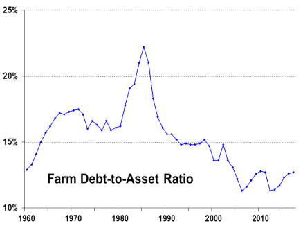
- The farm debt-to-asset ratio is forecast to be higher in 2017, at 12.7%, still a relatively low value by historical standards (Figure 24).
|
Measuring Farm Wealth A useful measure of the farm sector's financial wherewithal is farm sector net worth as measured by farm assets minus farm debt. A summary statistic that captures this relationship is the debt-to-asset ratio. Farm Assets include both physical and financial farm assets. Physical Assets include land and buildings, farm equipment, on-farm inventories of crops and livestock, and other miscellaneous farm assets. Financial Assets include cash, bank accounts, and investments such as stocks and bonds. Farm Debt includes both business and consumer debt linked to real estate and non-real-estate assets (e.g., financial assets, inventories of agricultural products, and the value of machinery and motor vehicles) of the farm sector. The Debt-to-Asset Ratio compares the farm sector's outstanding debt related to farm operations relative to the value of the sector's aggregate assets. Change in the debt-to-asset ratio is a critical barometer of the farm sector's financial performance with lower values indicating greater financial resiliency. A smaller debt-to-asset ratio suggests that the sector is better able to withstand short-term increases in debt related to interest rate fluctuations or changes in the revenue stream related to lower output prices, higher input prices, or production shortfalls. The largest single component in a typical farmer's investment portfolio is farmland. As a result, real estate values affect the financial well-being of agricultural producers and serve as the principal source of collateral for farm loans. |
 |
|
Source: NASS, Land Values 2017 Summary, August 2017. Notes: Farm real estate value measures the value of all land and buildings on farms. Cropland and pasture values are only available since 1998. All values are nominal (i.e., not adjusted for inflation). |
 |
|
Source: ERS, "2017 Farm Income Forecast," August 30, 2017. 2017 is a forecast. |
Average Farm Household Income
Farm household wealth is derived from a variety of sources.17 A farm can have both an on-farm and an off-farm component to its balance sheet of assets and debt. Thus, the well-being of farm operator households is not equivalent to the financial performance of the farm sector or of farm businesses because of other stakeholders in farming, such as landlords and contractors, and because farm operator households often have nonfarm investments, jobs, and other links to the nonfarm economy.
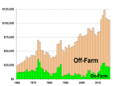
On-Farm vs. Off-Farm Income Shares
Average farm household income (sum of on- and off-farm income) is projected at $119,598 in 2017 (Table 2), up 1.4% from $117,918 in 2016 but well below the record of $134,164 in 2014.
About 20% ($24,262) of total household income is from the farm, and the remaining 80% ($95,336) is earned off the farm (including financial investments). The share of farm income derived from off-farm sources had increased steadily for decades but peaked at about 95% in 2000 (Figure 25).
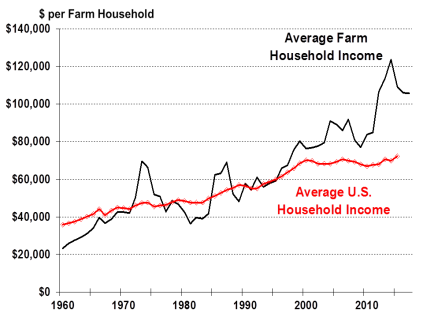
U.S. Total vs. Farm Household Average Income
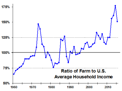
- Since the late 1990s, farm household incomes have surged ahead of average U.S. household incomes (Figure 26 and Figure 27).
- In 2015 (the last year for which comparable data were available), the average farm household income of $119,880 was about 51% higher than the average U.S. household income of $79,263 (Table 2).
Note on Aggregate Farm Household Data
Aggregate data often hide or understate the tremendous diversity and regional variation that occurs across America's agricultural landscape. This report focuses entirely on national aggregate statistics. It is not intended to identify or discuss significant differences that may occur across different production activities and regions. For insights into the potential diversity of differences in American agriculture, readers are encouraged to visit the ERS websites on "Farm Structure and Organization" and "Farm Household Well-being," where more information on such differences is readily available in a highly accessible format.18
|
Figure 27. U.S. Farm vs. Average Household Incomes Expressed as a Ratio |
 |
|
Source: ERS, "2017 Farm Income Forecast," August 30, 2017. 2015 is the last year with comparable data. |
USDA Monthly Farm Prices Received Charts
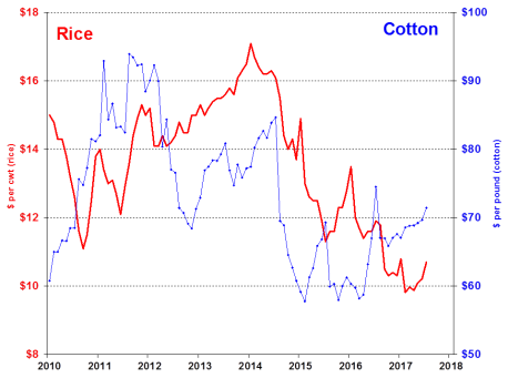
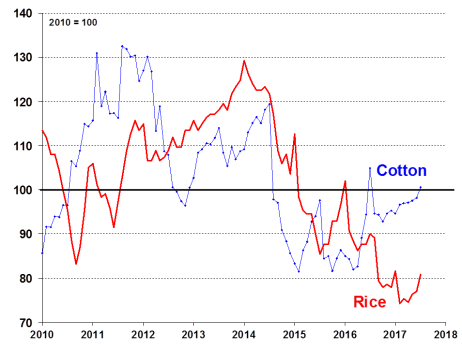
The following set of eight charts (Figure 28 to Figure 35) presents USDA data on monthly farm prices received for several major farm commodities—corn, soybeans, wheat, upland cotton, rice, milk, cattle, hogs, and chickens. The data is presented in both nominal and indexed formats to facilitate comparisons.
USDA Farm Income Data Tables
Three tables at the end of this report (Table 1 to Table 3) present aggregate farm income variables that summarize the financial situation of U.S. agriculture. In addition, Table 4 presents the annual average farm price received for several major commodities, including the USDA forecast for the 2016/2017 marketing year.
|
Figure 28. Monthly Farm Prices for Corn, Soybeans, and Wheat, Nominal Dollars |
 |
|
Source: USDA, National Agricultural Statistics Service (NASS), Agricultural Prices, August 30, 2017. |
|
Figure 30. Monthly Farm Prices for Cotton and Rice, Nominal Dollars |
 |
|
Source: USDA, NASS, Agricultural Prices, August 30, 2017. Notes: cwt = hundredweight or units of 100 lbs. |
|
Figure 34. Monthly Farm Prices for All Hogs and Broilers, Nominal Dollars |
 |
|
Source: USDA, NASS, Agricultural Prices, August 30, 2017. Notes: cwt = hundredweight or units of 100 lbs. |
|
Item |
2010 |
2011 |
2012 |
2013 |
2014 |
2015 |
2016 |
2017a |
Forecast Change (%) 2016 to 2017 |
||||||||||||||||||
|
1. Cash receipts |
|
|
|
|
|
|
|
|
|
||||||||||||||||||
|
Cropsb |
|
|
|
|
|
|
|
|
|
||||||||||||||||||
|
Livestock |
|
|
|
|
|
|
|
|
|
||||||||||||||||||
|
2. Government paymentsc |
|
|
|
|
|
|
|
|
|
||||||||||||||||||
|
Fixed direct paymentsd |
|
|
|
|
|
|
|
|
|
||||||||||||||||||
|
CCP-PLC-ARCe |
|
|
|
|
|
|
|
|
|
||||||||||||||||||
|
Marketing loan benefitsf |
|
|
|
|
|
|
|
|
|
||||||||||||||||||
|
Conservation |
|
|
|
|
|
|
|
|
|
||||||||||||||||||
|
Ad hoc and emergencyg |
|
|
|
|
|
|
|
|
|
||||||||||||||||||
|
All otherh |
|
|
|
|
|
|
|
|
|
||||||||||||||||||
|
3. Farm-related incomei |
|
|
|
|
|
|
|
|
|
||||||||||||||||||
|
4. Gross cash income (1+2+3) |
|
|
|
|
|
|
|
|
|
||||||||||||||||||
|
5. Cash expensesj |
|
|
|
|
|
|
|
|
|
||||||||||||||||||
|
6. NET CASH INCOME |
|
|
|
|
|
|
|
|
|
||||||||||||||||||
|
7. Total gross revenuesk |
|
|
|
|
|
|
|
|
|
||||||||||||||||||
|
8. Total production expensesl |
|
|
|
|
|
|
|
|
|
||||||||||||||||||
|
9. NET FARM INCOME |
|
|
|
|
|
|
|
|
|
Source: ERS, Farm Income and Wealth Statistics; U.S. and State Farm Income and Wealth Statistics, updated as of August 30, 2017.
a. Data for 2017 are USDA forecasts. Change represents year-to-year projected change between 2017 and 2016.
b. Includes Commodity Credit Corporation loans under the farm commodity support program.
c. Government payments reflect payments made directly to all recipients in the farm sector, including landlords. The non-operator landlords' share is offset by its inclusion in rental expenses paid to these landlords and thus is not reflected in net farm income or net cash income.
d. Direct payments include production flexibility payments of the 1996 Farm Act through 2001, and fixed direct payments under the 2002 Farm Act since 2002.
e. CCP = counter-cyclical payments; PLC = Price Loss Coverage; and ARC = Agricultural Risk Coverage.
f. Includes loan deficiency payments (LDP); marketing loan gains (MLG); and commodity certificate exchange gains.
g. Includes payments made under the ACRE program which was eliminated by the 2014 farm bill (P.L. 113-79).
h. Cotton ginning cost-share, biomass crop assistance program (BCAP), milk income loss (MILC), tobacco transition, and other miscellaneous program payments.
i. Income from custom work, machine hire, agri-tourism, forest product sales, and other farm sources.
j. Excludes depreciation and perquisites to hired labor.
k. Gross cash income plus inventory adjustments, the value of home consumption, and the imputed rental value of operator dwellings.
l. Cash expenses plus depreciation and perquisites to hired labor.
|
2010 |
2011 |
2012 |
2013 |
2014 |
2015 |
2016 |
2017F |
|||||||||
|
Average U.S. Farm Income by Source |
|
|
|
|
|
|
|
|
||||||||
|
On-farm income |
|
|
|
|
|
|
|
|
||||||||
|
Off-farm income |
|
|
|
|
|
|
|
|
||||||||
|
Total farm income |
|
|
|
|
|
|
|
|
||||||||
|
Average U.S. Household Income |
|
|
|
|
|
|
|
NA |
||||||||
|
Farm Household Income as Share of U.S. Avg. Household Income (%) |
125% |
|
156% |
|
177% |
151% |
NA |
NA |
Source: ERS, Farm Household Income and Characteristics, principal farm operator household finances, data set updated as of August 30, 2017, http://www.ers.usda.gov/data-products/farm-household-income-and-characteristics.aspx.
Note: NA = not available. Data for 2017 are USDA forecasts.
|
2010 |
2011 |
2012 |
2013 |
2014 |
2015 |
2016 |
2017F |
|||||||||||||||||
|
Farm Assets |
|
|
|
|
|
|
|
|
||||||||||||||||
|
Farm Debt |
|
|
|
|
|
|
|
|
||||||||||||||||
|
Farm Equity |
|
|
|
|
|
|
|
|
||||||||||||||||
|
Debt-to-Asset Ratio (%) |
|
|
|
|
|
|
|
|
Source: ERS, Farm Income and Wealth Statistics; U.S. and State Farm Income and Wealth Statistics, updated as of August 30, 2017, http://www.ers.usda.gov/data-products/farm-income-and-wealth-statistics.aspx.
Note: Data for 2017 are USDA forecasts.
|
Commoditya |
Unit |
Year |
2012/13 |
2013/14 |
2014/15 |
2015/16 |
2016/17 |
2017/18Fb |
% Change from 2016/17c |
2018/19Pb |
% Change from 2017/18d |
2017 Loan Ratee |
2017 Refer-ence Price |
|
Wheat |
$/bu |
Jun-May |
7.77 |
6.87 |
5.99 |
4.89 |
3.89 |
4.30-4.90 |
18.3% |
— |
— |
2.94 |
5.50 |
|
Corn |
$/bu |
Sep-Aug |
6.89 |
4.46 |
3.70 |
3.61 |
3.35 |
2.80-3.70 |
-4.5% |
— |
— |
1.95 |
3.70 |
|
Sorghum |
$/bu |
Sep-Aug |
6.33 |
4.28 |
4.03 |
3.31 |
2.85 |
2.50-3.30 |
1.8% |
— |
— |
1.95 |
3.95 |
|
Barley |
$/bu |
Jun-May |
6.43 |
6.06 |
5.30 |
5.52 |
4.96 |
4.20-5.20 |
-5.2% |
— |
— |
1.95 |
4.95 |
|
Oats |
$/bu |
Jun-May |
3.89 |
3.75 |
3.21 |
2.12 |
2.06 |
2.25-2.75 |
21.4% |
— |
— |
1.39 |
2.40 |
|
Rice |
$/cwt |
Aug-Jul |
15.10 |
16.30 |
13.40 |
12.10 |
10.30 |
12.70-13.70 |
28.2% |
— |
— |
6.50 |
14.00 |
|
Soybeans |
$/bu |
Sep-Aug |
14.40 |
13.00 |
10.10 |
8.95 |
9.50 |
8.35-10.05 |
-3.2% |
— |
— |
5.00 |
8.40 |
|
Soybean Oil |
¢/lb |
Oct-Sep |
47.13 |
38.23 |
31.60 |
29.86 |
32.50 |
32.50-36.50 |
6.2% |
— |
— |
— |
— |
|
Soybean Meal |
$/st |
Oct-Sep |
468.11 |
489.94 |
368.49 |
324.6 |
315 |
290-330 |
-1.6% |
— |
— |
— |
— |
|
Cotton, Upland |
¢/lb |
Aug-Jul |
72.5 |
77.9 |
61.3 |
61.2 |
68 |
54-66 |
-11.8% |
— |
— |
45-52 |
none |
|
Choice Steers |
$/cwt |
Jan-Dec |
122.86 |
125.89 |
154.56 |
148.12 |
120.86 |
118-120 |
-1.5% |
111-120 |
-2.9% |
— |
— |
|
Barrows/Gilts |
$/cwt |
Jan-Dec |
60.88 |
64.05 |
76.03 |
50.23 |
46.16 |
50-51 |
9.4% |
46-50 |
-5.0% |
— |
— |
|
Broilers |
¢/lb |
Jan-Dec |
86.6 |
99.7 |
104.90 |
90.5 |
84.3 |
93-95 |
11.5% |
85-92 |
-5.9% |
— |
— |
|
Eggs |
¢/doz |
Jan-Dec |
117.4 |
124.7 |
142.3 |
181.8 |
85.7 |
87-89 |
2.7% |
87-94 |
2.8% |
— |
— |
|
Milk |
$/cwt |
Jan-Dec |
18.53 |
20.05 |
23.97 |
17.12 |
16.30 |
17.70-17.90 |
9.2% |
17.55-18.55 |
1.4% |
— |
— |
Source: Various USDA agency sources as described in the notes below.
a. Season average farm price for grains and oilseeds are from USDA, National Agricultural Statistical Service, Agricultural Prices. Calendar year data are for the first year, for example, 2017/2018 = 2017; F = forecast and P = projection from World Agricultural Supply and Demand Estimates (WASDE) September 12, 2017;—= no value; and USDA's out-year 2017/2018 crop price forecasts will first appear in the May 2017 WASDE report. Soybean and livestock product prices are from USDA, Agricultural Marketing Service (AMS): soybean oil—Decatur, IL, cash price, simple average crude; soybean meal—Decatur, IL, cash price, simple average 48% protein; choice steers—Nebraska, direct 1100-1300 lbs; barrows/gilts—national base, live equivalent 51%-52% lean; broilers—wholesale, 12-city average; eggs—Grade A, New York, volume buyers; and milk—simple average of prices received by farmers for all milk.
b. Data for 2017/2018 are USDA forecasts; 2018/2019 data are USDA projections.
c. Percent change from 2016/2017, calculated using the difference from the midpoint of the range for 2017/2018 with the estimate for 2016/2017.
d. Percent change from 2017/2018, calculated using the difference from the midpoint of the range for 2018/2019 with the estimate for 2017/2018.
e. Loan rate and reference prices are for the 2017/2018 crop year. See CRS Report R43076, The 2014 Farm Bill (P.L. 113-79): Summary and Side-by-Side.